Site map/guide to tutorials Contact | News Making fine prints in your digital darkroom Understanding image sharpness and MTF Image galleries / How to purchase prints Photographic technique Image editing with Picture Window Pro A simplified zone system Digital vs. film

View image galleries

Search WWW Search www.normankoren.com

If you are unfamiliar with MTF, you may want to review Part 1 of the Understanding image sharpness series.

Dennis Wilkins' comparison of the Nikon D100 with Reala film

---

My friend Dennis Wilkins, who recently took early retirement as a quality control guru at Hewlett-Packard, took time off from his busy consulting schedule to perform the following comparison between his new Nikon D100 digital (23.7x15.6 mm sensor; 1.52x focal length multiplier) and his traditional Nikon N70. The test chart, made years ago by Paterson Photographic Ltd., is apparently long out of production. Here are his comments, slightly edited. Same lens (Nikkor 24-120mm @ 50 mm), same f-stop (f/11), same tripod, same brand of camera (Nikon), N70 with Fuji Reala at ISO 100 vs. D100 at ISO 200 (sorry, it goes no lower). D100 shot at 1:39 ratio, N70 shot at 1:26 ratio in order to make the overall image scale the same due to 1.5:1 lens multiplier. Thus, everything is the same except the focusing distance, which should have little effect on resolution. (The lens is not the limiting factor here.) 1. Reala, ISO 100, scanned on a Canon FS4000 at 4,000 dpi, no extra sharpening. (The Canon has built-in sharpening that can't be turned off). 2. D100, ISO 200, normal sharpening. The scale actually represents approximately 7.5 to 75 lines per mm (that 1.5x multiplier). 3. Reala, ISO 100, same scan as 1, with extra sharpening . Film images 1 and 3 have more grain than 2, with more grain visible in 3 due to sharpening. The mottling of the cyan ink in digital image 2 resembles the target itself (the black, yellow and magenta have smoother ink coatings). The D100 image appears sharper than even the extra sharpened Reala/Canon scan. These are at 1:1 for the D100 scale (I had to adjust scales because the D100 imager is only 70% the dimensions of 35mm) and represent a section of an enlargement that would be 28" x 42". I tried (not totally successfully) to make the tones the same. The D100 resolution chart shows some moiré interactions down in the 30-35 lp/mm range (which is really not that value at the actual D100 scale -- it's really more like 45-50 lp/mm). Note this Moiré effect is rarely of concern because most real photos don't contain such precise, repetitive, high-contrast pitch elements. (It could be a problem with fabrics in fashion photography-- NK). Dennis's comparison of the D100 vs. the 10D can be found on my 10D page.  My (NLK) observations: The D100 has higher contrast up to nearly 30 on the scale (roughly 45 lp/mm) and much less noise (grain). Response above 30 is mostly artifacts. Reala scanned at 4000 dpi has resolvable detail to over 35, but contrast is very low above about 28 and the image is noticeably grainy. Overall image quality looks better with the D100. These tests agree reasonably well with my simulation results.

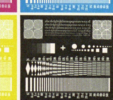
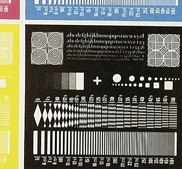
1. Reala, ISO 100, 1:26, 4000 dpi scan. 2. D100, ISO 200, 1:39, normal sharpening. 3. Reala, ISO 100, 1:26, 4000 dpi scan, extra sharpening.

The future of digital cameras

---

• Compact digital cameras with sensors up to 11 mm diagonal come in several varieties, usually with one or more dominant features, such as
• Basic low-cost point-and-shoot
• Ultra-compact
• Large aperture lens
• Large zoom ratio (up to 12:1) with long telephoto
• High pixel count (6+ megapixels)
  

11 mm diagonal sensors are very small-- 1/4 the length and 1/16 the area of a 35mm frame, and many of these cameras have smaller sensors. But most are sharp enough to make outstanding 8½x11 inch prints, and many can make decent 13x19 inch prints. Prosumer sensors seem to be stabilizing at around 6-8 megapixels. The Pixel spacing for typical 8 megapixel sensors is tiny-- 2.7 µm vs. 3.4 µm for 5 megapixel sensors. Noise can be relatively high (especially at ISO speeds greater than 100) and exposure range is limited. But resolution seems to be excellent-- better than the 5 megapixel models. I believe 8 megapixels is about as far as compact digital cameras are likely to go; they require fine (i.e., expensive) lenses to reach their potential. More (smaller) pixels would be noisier and offer little advantage in resolution, which would be limited by lens quality and diffraction. There will be progress in other aspects of sensor performance. For example, Fuji's new Super CCD SR promises increased exposure (dynamic) range. Progress in compact digital cameras won't be as dramatic as it was before 2004; it will consist of more refined feature sets, better battery life, less shutter lag, wireless communications, and lower cost-- a relief to those who worry about their investments becomming obsolete overnight.

• Digital SLRs with sensors smaller than full-frame 35mm (22-28 mm diagonal). These include cameras with APS-C-sized sensors (around 27mm diagonal), such as the Nikon D50, D70, and D100, and the Canon EOS-20D and Digital Rebel, and the Olympus-Kodak Four-thirds inch initiative (22 mm diagonal sensors), with the Olympus E-1 as the flagship. These cameras are a compromise between compacts, which can be noisy and have a limited exposure range, and full-frame 35mm sensors, which are far more expensive: Sensor cost increases rapidly with size, scaling with at least the third power of sensor area.
  
  At first I thought these cameras were a stopgap measure on the way to full-frame cameras. I was wrong. They're here to stay. Compared to the full-frame cameras, they are much less expensive and slightly smaller and lighter. Several manufacturers (Canon, Nikon, Sigma, Tamron, Tokina) now make lenses for this format. These lenses are sharper, smaller, and lighter then their counterparts that cover the full 35mm frame. The image quality in the best of these cameras equals 35mm: I can make better 13x19 inch enlargements with my Canon EOS-20D than I've ever seen from 35mm.
  
  There cameras will continue to evolve: pixel count will increase, topping out at around 12 megapixels, and feature sets will improve. Wireless technology will become commonplace. But don't expect anything really dramatic. I have some doubts about the Four-thirds standard. The Olympus cameras are technically excellent, but there is no upward migration path for photographers who want to upgrade to full frame cameras.
  
  
• Digital SLRs with full-frame 35mm (44 mm diagonal) sensors are the cameras of choice for professionals and serious amateurs who can afford them. The best of them-- the Canon EOS-1Ds Mark II-- has image quality comparable to medium format film (645). The recently-announced EOS 5D comes close, and it is smaller, lighter, and less expensive. The number of pixels in full frame cameras will slowly increase, topping out around 24 megapixels. There would be little benefit from more pixels: resolution would be limited by the lens, and noise, dynamic range, and yield would deteriorate. Prices will continue to drop as sales and sensor manufacturing yields increase. I am considering the purchase of and EOS 5D in 2006.
  
  
• Cameras/backs with sensors larger than 44 mm diagonal. Very expensive; primarily of interest to professionals. An example is the 22 megapixel Sinarback 54, which uses the Kodak KAF-22000CE CCD image sensor: 4080 x 5440 pixels, 9 µm pixel spacing, about 36x48 mm image size-- twice that of 35mm and close to full frame 645 medium format. It is capable of making sharp 24x32 inch prints. If you have to ask the price... See Michael Reichmann's Survey of Current Medium Format Digital Backs. I'll pay more attention if and when they become affordable (or I strike it rich).

The handwriting is on the wall for film. 16 megapixel sensors (10 for the X3 sensor, if they can produce it) have resolution challenging medium format film. Large users of film have already switched to digital. Film sales are rapidly dropping. Film production lines will shut down as sales drop. Variety will decrease and prices will increase. Traditionalists will complain, but the quality of digital images will carry the day. At 16 megapixels, many traditional view camera applications are migrating to digital, where they can take advantage of Canon and Nikon tilt-shift lenses that turn 35mm/digital cameras into baby view cameras.

Moore's law for semiconductors (named for Gordon Moore, co-founder of Intel) states that the complexity of silicon chips doubles approximately every 18 months. For years digital sensors progressed more slowly, but the growing market sped up progress between 1998 and 2003-- the 3.11 megapixel Canon EOS D30 was followed by the 6.3 megapixel D60 in about 18 months and the 11 megapixel EOS-1Ds a year later. However Moore's law applies primarily to digital logic chips, which keep shrinking, whereas digital sensor pixels can't shrink indefinitely. Quality is diminished-- film speed and exposure range and noise get worse-- as pixel size decreases. Pixel spacings below 5 µm probably won't meet professional standards; the gain in resolution won't be sufficient to compensate the increased noise and decreased exposure range. For high quality imaging, pixels will remain in the optimum 6-9 µm range, and sensor sizes will be APS-C or larger.

Supporting technologies-- flash memories and microdrives-- will continue to advance with the speed of Moore's law. Image processing workflows for both amateurs and professionals will improve-- driven by huge potential profits. New wireless technologies will allow images to be uploaded from cameras in near-realtime: Bluetooth, for devices within 10 meters, and Qualcomm's third-generation data-optimized wireless technology (1xEV-DO). Either of these will boost a camera's storage capacity to near-infinite--no more changing film or PC cards. Uploads can be done in the background without intervention by the photographer-- the possibilities are quite staggering.

Thom Hogan has some interesting prognostications in What Will Happen in 2004? (His What Will Happen in 2003? is also very interesting. This link may be behind...)

Links

---

George Nyman has created a very clear comparison between digital and film:  Brief Comparison of CANON 20D, NIKON D70S, CANON 1D MkII, PENTAX *istDS, K-MINOLTA D7, Fuji S3Pro and NIKON D2X with FILM (35mm, 4,5x6,6x6, 6x8).

Peter Wolff's clear comparison of the EOS-1Ds with 35mm and medium format in Photographical.net (excellent site) is most interesting. Summary (no surprise): The EOS-1Ds trounces 35mm and seriously challenges medium format.

Scientific test report comparing current digital cameras with 35mm SLR film cameras by Anders Uschold. Contains experimental data on the Canon D60, Nikon D100 and Fuji S2 Pro. Examines the interaction of lenses and digital sensors with data from several excellent lenses. Translated from German; awkward in places. Related articles covering testing techniques are available in German; they will be added to the English language pages in the next few months. Anders organized a symposium on Digital image capture – Camera testing and quality assurance at Photokina 2002. The PDF presentations, covering resolution, dynamic range and image quality issues, are extremely interesting. I would love to see full text versions.

Optics for digital photography  A white paper from Schneider Optics. Rather poorly written-- some of the numbers assume you would never enlarge more than 7.5x11 inches (A4), but interesting nonetheless. Outlines lens design goals for digital cameras: Maintain high MTF to some fraction of the Nyquist frequency (RMAX = 1/(2*pixel spacing)), then have MTF drop as rapidly as possible so the MTF of the lens+sensor (calculated in the tables above) at Nyquist is no more than about 10%. This keeps aliasing under control. Figure 2 has a glaring error: edges in the brightness distribution would be softened by the MTF response. The middle and right would resemble sine waves.

Sony CCD data sheets  Some of their sensors are as small as 5 mm diagonal (35mm is 43.3 mm diagonal). The Sony DSC-F707 uses one of the 11 mm diagonal 5.07 Megapixel ICX282 series sensors. Pixel length is a tiny 3.4 µm. No anti-aliasing filter is needed. These tiny pixels have more noise and less dynamic range than larger (over 6 µm) pixels.

Kodak image sensor solutions  Links to technical information and valuable articles. Their high-end sensors are the KAF Blue Plus Color Series. The sensor for the Kodak DCS 14n is made by The Fill Factory.

Fairchild Imaging's CCD595 CCD sensor has 85 Megapixels !!!  9216x9216 8.75 µm pixels; 8.064 cm².  It's designed for aerial reconnaissance. My budget is a bit smaller than the Pentagon's (as is my deficit), but I can always dream.

Film versus Digital Cameras by Robert Monaghan. Heated debate punctuated by some valuable technical information.

Roger N. Clark, Ph.D. in Planetary Science from MIT and avid photographer, has some valuable information on digital resolution. His recent page on Film vs. digital has some interesting comments on dynamic range, which is superb with digital.

Ken Rockwell's views on digital vs. film are based on his experience in the film industry. I disagree with many of his statements, but when when you compare 4x5 film to a 6 megapixel DSLR, what's to disagree, duh?

Tawbaware.com has done a nice little film vs. digital test-- a good reality check on my calculations.

ST Microelectronics (UK) has some interesting technical pages on CMOS sensors.

Horst Kretzschmar ( www.eos-d60.de ) is planning a series of lens tests on the Canon EOS D60 using my lens test charts.

Anatomy of a Digital Camera: Image Sensors from Extremetech.com.

Canon Digital Photography Forum (not an official Canon site)  Excellent discussion forum.

Digital Images: Foveon X3 versus Bayer by Mike Chaney of Qimage Pro  A nice simulation illustrating the superiority of the Foveon sensor.

RIT Center for Imaging Science class material is a serous resource-- well worth exploring. Basic Principles of Imaging Science 1. Lectures 17 and 18 on MTF and imaging microstructure are particularly interesting.

Mikhail "Teddybear" Sokolov has some interesting material comparing the Fuji S2 Pro digital SLR with film and other digital cameras. Mostly Russian, but this link is good for translations. See two dpreview.com posts: The most over asked question (image comparisons) | Fuji SLR Talk (chart comparisons)
.

Measuring MTF from ISO 12233 charts Both dpreview.com and imaging-resource.com publish test images of the ISO 12233 test chart. With the procedure below you can use them to estimate the 50% MTF frequency. But it's rather tedious. The new Imatest program provides far more convenient and accurate MTF measurements. Several portions of the ISO 12233 resolution test chart are typically printed on the last "Image Quality" or "Compared to..." page in each dpreview.com test report. A portion of the EOS D30 chart is shown on the right. You can download and save complete resolution charts (as large, high quality JPEGs) by right-clicking on any of the reduced or cropped images. On imaging-recource.com, the chart can be found on the Sample images pages. To analyze a chart, load it into a program such as Pixel Profile or ImageJ, described below, that allows you to measure the following values. Image editors can also be used, but they're less convenient. VB The average luminance for black areas. VW The average luminance for white areas. Vmin The minimum luminance for a bar pattern at a given frequency or scale value (the "valley" or "negative peak"). Vmax The maximum luminance for a bar pattern at a given frequency or scale value (the "peak"). Use the following equations to find MTF. C(0) = (VW-VB)/(VW+VB) is the low frequency (black-white) contrast. Contrast defined in this way, normalized to (divided by) (VB+VW),  minimizes errors due to nonlinearities in acquiring the pattern. C(f) = (Vmax-Vmin)/(Vmax+Vmin) is the contrast at spatial frequency f. MTF(f) ~= 78.5%*C(f)/C(0), where C(f) < 0.7*C(0)  The 78.5% factor is explained in the box below. . Approximating MTF   MTF is based on sine wave response, but we often work with bar charts. The contrast ratio obtained directly from a bar chart is called the contrast transfer function, CTF(f) = 100% * C(f) / C(0). CTF is rarely referred to in the literature. It is not the same as MTF. A portion of a bar chart can be approximated by a periodic function called a square wave, illustrated above for period 2L (frequency = f = 1/2L). Fourier transform mathematics teaches us that any periodic function can be expressed as an infinite sum of sine functions, starting with the fundamental, sin(pi*x/L) = sin(2*pi*f), and including harmonics, sin(n*pi*x/L) = sin(2*n*pi*f) for n = 2, 3, 4, ... The equation for the square wave is shown above. It only has odd harmonics (n = 3, 5, 7,...). The amplitude of the fundamental frequency of the bar pattern is 4/pi = 1.273 times the amplitude of the bar pattern itself. To obtain MTF from CTF you must multiply by a factor of pi/4, hence, MTF(f) = 0.785*CTF ~= 78.5%*C(f)/C(0),  where C(f) < 0.7*C(0) This equation is only accurate at relatively high frequencies where response is dropping-- where the harmonics are strongly attenuated. These are the frequencies of interest. The exact equation for relating MTF(f) to CTF(f) was given by Coltman (1954): MTF(f) = pi/4 * [CTF(f) + CTF(3f)/3 - CTF(5f)/5 + CTF(7f)/7 ...] The signs in this equation beyond n  = 7 are quite irregular. This equation is rarely of practical interest-- pure geek stuff. I owe thanks to Chuck Varney for straightening me out on these issues. There two basic ways to analyze the chart. 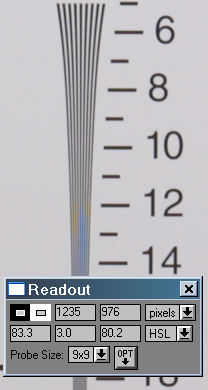Load the saved chart into an image editor that has a readout tool. A portion of the chart for the Canon EOS D30 is shown above, along with the Picture Window Pro readout tool. Zooming in larger that 1x (one screen pixel per image pixel) allows a clearer look at the chart. In PW Pro, bring up the readout tool by clicking Tools, Readout, and select HSL. The default probe size is 3x3 pixels: change it to 1x1 for MTF measurements. Observe the average luminance (L in HSL) for black and white areas, VB and VW. A large probe size (up to 9x9) makes this easier. For the D30 chart (on the right), VB = 18% and VW = 80%. (100% = pixel level 255.) C(0) = (VW-VB)/(VW+VB) = 0.633. Now zoom in on the portion of the chart shown, located near the right-center. Set the probe size to 1x1 pixels. Run the probe across the pattern at some point on the scale, looking for the average minimum and maximum values, Vmin and Vmax. It may take a while to get the hang of it. For the D30 chart at scale = 10 (about 33 lp/mm), Vmax ~= 65% and Vmin ~= 43%. C(f) = (Vmax-Vmin)/(Vmax+Vmin) = 0.204. MTF(scale=10) ~= 78.5%*C(f)/C(0) = 25%. This technique is only as good as your estimate of Vmax and Vmin: maybe about ±10%. The technique below is slightly more accurate. Use a program that plots image pixel luminance. PixelProfile is easy to use; its operation is largely self-explanatory, but it is limited to 640x480 pixel image size; you'll want to crop the image and save it as a maximum quality JPEG before loading it. ImageJ is more versatile-- it can handle larger images. A PixelProfile intensity plot (same as  HSL Lightness) is shown below for the D30 chart at scale = 10 (about 33 lp/mm). VW = 207, VB = 45, Vmax = 167, and Vmin = 115 (Vmax and Vmin are both averages). Plugging into the above equations, C(0) = 0.643, C(scale=10) = 0.184, MTF = 78.5%*0.184/0.643 = 22%. This approach is slightly more accurate than the first approach. The scale on the chart is the number of line widths per picture height divided by 100, 00 has been dropped to save space. For example, 12 represents 1200 lw/ph. But line pairs are universally used in MTF charts, and it takes two lines (line widths) to make one line pair. To get the total line pairs for the chart height, multiply the scale by 50. A value of 12 equates to 600 line pairs per picture height. The equation for line pairs per mm is lp/mm = scale*50/(picture height in mm) Dpreview.com's test pages state, "Values on the chart are 1/100th lines per picture height. So a value of 8 equates to 800 lines per picture height." The resolution page states, "Resolution from this chart is always measured in lines per picture height (to keep the pixels square), the numbers seen on the chart refer to hundreds of lines, so the label "12" refers to 1,200 lines per picture height." The use of line width instead of line pairs is an old standard, still used by PIMA / IT10 to measure TV resolution. It can be confusing because it differs from the spatial frequency in MTF charts by a factor of 2. At MTF = 50%, C(f)/C(0) = 0.637; at MTF = 10% C(f)/C*0) = 0.127. Little sharpening is evident for the 15.1mm high D30 sensor (above). The Moiré and checkerboarding between 12 and 15 ( 40 and 50 lp/mm) are caused by the Bayer pattern interpolation routines. Sharpening in the image editor boosts MTF frequencies, but, as always, sharpening comes at a price. It makes high frequency artifacts--Moiré and checkerboarding-- more visible. Pixel Profile display for Intensity (L in HSL representation) for a section of the above chart at scale = 10, corresponding to 10*50/15.1 mm  = 33.1 lp/mm. The period of the pattern is (32-8.5)/8 = 2.94 pixels per line pair. The 0.0102 mm pixel spacing of the D30 corresponds to a period of 0.0300 mm, or 33.4 lp/mm. Close enough.

Images and text copyright © 2000-2013 by Norman Koren. Norman Koren lives in Boulder, Colorado, where he worked in developing magnetic recording technology for high capacity data storage systems until 2001. Since 2003 most of his time has been devoted to the development of Imatest. He has been involved with photography since 1964.