Understanding image sharpness part 1A:
Resolution and MTF curves in film and lenses
by Norman Koren

---

Site map/guide to tutorials Contact | News Making fine prints in your digital darkroom Understanding image sharpness and MTF Image galleries / How to purchase prints Photographic technique Image editing with Picture Window Pro A simplified zone system Digital vs. film

View image galleries

Search WWW Search www.normankoren.com

In this page we illustrate how MTF is used to characterize the performance of film and lenses.

Film

---

Digital photographers may skim this section quickly. Many of the films have been discontinued.

The curve on the left is the MTF for Kodak E100VS reversal (slide) film (similar to Elite Chrome 100). A different MTF is shown for each color layer: red, green, and blue (R, G, and B). Green is the most important because the eye is far more sensitive to it than to other colors. The green curve is close to the MTF curve for Fujichrome Provia 100F. Most film MTF curves can be closely approximated by a function known as the Lorentzian, MTFfilm( f ) = 1/(1+( f/f50)2) f  is frequency;  f50 is the frequency where MTF = 0.5 = 50%. For the E100VS green layer,  f50 = 40 line pairs/mm. For the mathematically challenged, MTF( f ) is expressed in functional notation, which indicates that MTF is a function of frequency,  f.

Electrical engineers will note that this curve has a second order Butterworth response. Second order means that at high frequencies,  f >> f50, response drops twice as fast as frequency increases; it is proportional to 1/ f 2. This is also called this a 12 dB (decibels) per octave rolloff (6 dB per octave per order). The MTFcurve program illustrates the effects of MTF on the input target. MTF is applied only in the horizontal direction (it's two dimensional in actual images). The blue curve below the target is the film MTF, expressed in percentage-- the scale on the left applies. It closely approximates the green curve for Ektachrome E100VS. The red curve shows the density of the bar pattern. The 50% and 10% amplitudes are 40 line pairs/mm, as expected, and 120 line pairs/mm. This plot is generated from Matlab by entering MTFcurve2 40

The MTF curve on the left is from an old data sheet for Fujichrome Velvia, a highly saturated ASA 50 slide film known for its sharpness. Something is different here: a boost in the MTF response, which peaks at around 125% at 10 line pairs/mm. What can this mean? From my former career, I recognized this curve as characteristic of pulse slimming equalizers, widely used in older magnetic disk drives to sharpen readback pulses so more data can be squeezed into a given area. By adding one more parameter, fboost, I was able to fit it reasonably well. MTFfilm( f ) = k / (1+(( f - fboost) / f50a )2) fboost is the frequency of maximum MTF. The percentage boost depends on the ratio,  fboost / f50. fboost must be less than  f50 /2. k is a constant set so that MTF(0) = 1. One caution about this equation: it rolls off more rapidly at high spatial frequencies ( f >> f50) than the equation without fboost (or fboost = 0). This boost is called the adjacency effect boost for reasons described below. It is similar in nature to the boost caused by digital sharpening.

f_50a =  sqrt( f₅₀²-2 f₅₀ f_boost - f_boost²) so that  f₅₀ (as entered in MTFcurve) is still the 50% MTF frequency.

The striking feature of the response, shown in the red curve below the image, is the exaggerated contrast boundaries. Tones overshoot their low frequency (steady state) levels, and the result is plainly visible. The overall effect is that this image appears slightly sharper than the image above for Ektachrome E100VS or Fuji Provia 100F, even though it has slightly lower response at 100 line pairs/mm.

This effect is similar to the sharpen or unsharp mask functions in image editing programs.

There is a fairly elementary explanation of how this happens in film. It it particularly noticeable with black & white films developed in highly diluted (one-shot) developers. Visualize a contrast boundary between two areas, one side of which is heavily exposed (a highlight) and the other lightly exposed (a shadow). As the film is developed (particularly in the interval between between agitations), the developer in the heavily exposed area becomes depleted more rapidly than the developer in the lightly exposed area, slowing down the development. Some of the developer diffuses across the boundary, so that the developer in the heavily exposed area adjacent to the boundary is less depleted than in the rest of the region, hence develops more rapidly, and the developer in the lightly exposed area adjacent to the boundary is more depleted, hence develops more slowly. The result is an exaggerated contrast boundary, as illustrated above. This is known as the adjacency effect, and film/developer combinations that exhibit it are said to have high acutance. In Velvia, the diffusion probably takes place inside the film.

The adjacency effect increases the perceived image sharpness, though it can become irritatingly obvious if it's overdone. It boosts the the MTF 50% frequency, but it has relatively little effect on the 10% level, which is related to perceived line pairs per mm resolution. Developing technique affects MTF, particularly for B&W films, where there is a large choice of developers and agitation procedures. Development options are more limited for color films.
 

View image galleries  . . An excellent opportunity to collect high quality photographic prints and support this website .

Is color negative film sharper? If you choose to believe manufacturer's data sheets, yes, they are sharper. Thanks to Mitch Mirkin and Jussi Ikäheimo for pointing out data I'd missed. MTF data for Fujicolor Superia 100 color negative film is shown on the right. f50 is around 63 lp/mm. That's about 50% better than Fuji's highly regarded Provia 100F slide film. (Curiously, resolving power, which has less to do with perceived sharpness, is about the same.) Kodak color negative films show a comparable improvement, for example, about 72 cycles/mm for Ultra Color 100UC vs. about 38 cycles/mm for Kodachrome 64 and 40 cycles/mm for Elite Chrome 100 and Chrome Extra Color 100. MTF for Kodak Gold films (Farbwelt in German) are shown on the Kodak Germany site. For Gold 100, shown below,  f50 (extrapolated) is about 110 lines/mm with a 40% adjacency effect boost. (Thanks to Stefan Ittner for directing me to the Kodak Germany site.) This evidently means line widths.  f50 expressed in the more familiar line pairs (or cycles) per mm would be 55.  . . 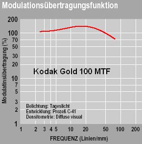Take this data with a grain of salt. I have limited evidence that color negatives are actually sharper. Andreas Kaseder published a small comparison of ASA 100 films (part of his Nikon 4000 ED review) that seems to indicate that negative film is sharper but grainier. I've made amazingly sharp prints of the Aspens on the Pitkin Creek trail, taken with Kodacolor Gold 100. The likely reason that slide film has poorer sharpness is that it's made to be displayed directly. Dark tones must be deep and rich; Dmax is much higher than for negative films, hence more dye is needed. Emultion layers may have to be thicker to accomodate this. . . Why then do slide films have such a good reputation? Mostly because they have finer grain (and also because traditional printing loses some sharpness). Remember, sharpness and grain are not the same thing, although both affect image quality. With B&W films you could trade them off with your choice of developer: Microdol-X had the finest grain; Rodinal was the sharpest but grainiest. Camera store/drugstore prints can't begin to do justice to the information stored on negatives. You need a scan, perferably 4000 dpi. As we mentioned earlier,  MTF (sharpness) corresponds to the bandwidth of a communications system while grain corresponds to its noise. Both enter into Shannon's equation for information transmission capacity, C = ω log2(SNR+1) where C is capacity, ω is bandwidth, and SNR is the signal-to-noise power ratio (drops as grain increases). I suspect that the tradeoff between grain and sharpness doesn't have much effect on capacity-- perceived image quality may be more a function of C than of either grain or sharpness by themselves. This, of course, is mostly speculation. I'll return to this topic in the discussion of image quality in Digital cameras vs. film

Film links and MTF data

---

Kodak publishes MTF data for some color reversal and B&W negative films. Go to Kodak Professional Products or Kodak Consumer Products- Film and navigate from there. Searching for MTF on Kodak's main page also works well. Kodak Germany publishes MTF curves for Gold films, called Farbwelt in German. Ektachrome E200 has f₅₀ = 34 lp/mm. Kodak T-MAX 100 has f₅₀ = 125 lp/mm and T-MAX 400 has f₅₀ = 100 lp/mm with 20% boost. T-MAX P3200 has f₅₀ = 85 lp/mm. These MTF's are quite striking-- far beyond any color reversal film! Photodo's page on 35 mm, medium format, or large format? indicates that T-MAX 100 is indeed a remarkable film. 35 mm T-MAX 100 outperformed medium format Tri-X using very fine equipment. Photodo's articles are worthy of serious study. Kodak also uses a measurement called print grain index for prints.

Fujifilm publishes MTF data for all their films. Go to Consumer Film Product Line-up or Professional Film Product Line-up and navigate from there. Fujicolor NHGII ASA 800 and NPH 400 color negative films have f₅₀ = 45 lp/mm.

There is one troubling aspect to some manufacturer's MTF curves, for example Fujichrome Provia 100F. MTF should be 100% at very low frequencies, but it remains flat at 120% from 10 lp/mm down to 1 lp/mm. There are three possible reasons. (1) The adjacency effect extends to extremely low spatial frequencies. Doubtful. 1 lp/mm is awfully low. (2) The graphic arts department took liberties with the plot before sending it out for publication. This happened to me in the old days before I had access to computer tools. (3) The marketing department cheated. It happens.

The Imatest program allows you to measure the MTF of digital cameras or digitized film images. You can't measure an individual component in isolation, but you can compare components, such as lenses, with great accuracy. Imatest also measurs other factors that contribute to image quality.

Lenses

---

The MTF curves on the right are from the Photodo (old site) test of the Canon 28-70mm f/2.8L lens. Photodo is an outstanding Internet lens test resource, with 458 lenses optically MTF tested as of June 2000. Photodo curently uses Imatest for its lens tests. In their page, Understanding the MTF graphs, numbers and grades, they state,

"The graphs show MTF in percent for the three line frequencies of 10 lp/mm, 20 lp/mm and 40 lp/mm, from the center of the image (shown at left) all the way to the corner (shown at right). The top two lines represent 10 lp/mm, the middle two lines 20 lp/mm and the bottom two lines 40 lp/mm. The solid lines represent sagittal MTF (lp/mm aligned like the spokes in a wheel). The broken lines represent tangential MTF (lp/mm arranged like the rim of a wheel, at right angles to sagittal lines). On the scale at the bottom 0 represents the center of the image (on axis), 3 represents 3 mm from the center, and 21 represents 21 mm from the center, or the very corner of a 35 mm film image. Separate graphs show results at f8 and full aperture. For zoom lenses, there are graphs for each measured focal length."

They state elsewhere that performance at 10 line pairs/mm is indicative of the lens contrast while 40 line pairs/mm is indicative of its sharpness.

Lens performance is typically limited by aberrations at large apertures and diffraction at small apertures. Aberrations depend on lens design and manufacturing quality; they differ markedly for different lenses. Diffraction is a fundamental physical effect; it depends on the aperture alone. A lens is sharpest between the two extremes, near its optimim aperture, which tends to be around f/8 or f/11 for the 35mm format. It is smaller (as low as f/4) for compact digital cameras and larger (f/11 to f/22) for large format cameras.

Unlike film, the MTF of lenses don't necessarily match the second order 1/(1+( f / f₅₀)²) equation. MTF rolloff can vary widely, depending on lens design and manufacturing tolerance. To accommodate this, MTFcurve has an input variable for the order of the lens's MTF rolloff, lord, which defaults to 2 if not entered or if entered as 0. The lens MTF equation becomes,

MTF_lens(f) = 1/(1+|f/f_lens|^lord)    (lord defaults to 2 in MTFcurve if not entered)

The Canon 28-70mm f/2.8L lens in this test is an outstanding performer, achieving a Photodo rating of 3.9 out of a possible 5, about as good as zoom lenses for the 35mm format (covering 43mm diagonal) get. At 40mm, f/8, it's as sharp as a first rate prime (single focal length) lens. With MTF40 around 70% at f/8, flens is around 61 line pairs/mm The down side: it's expensive (over $1000 US), large, and heavy. But sharp. The photo.net review is full of hypebole like, "one *bleeping* sharp zoom!," "sharpness and contrast is spectacular," "a stunning piece of glass," etc. Since 35mm lenses don't get much better I use this lens as the standard for the "excellent 35mm lens" for the remainder of this article. The plot on the right, generated by MTFcurve2 45 13 61 shows the combined response of Velvia film and the excellent 35mm lens. The red curve is the spatial response, the blue curve is the combined MTF, and the thin blue dashed curve is the MTF of the lens only. The 50% and 10% points for MTF are now 36.8 and 68.6 line pairs/mm. This is the best that can be expected for an excellent lens covering 43mm diagonal, optimum aperture, correct focus, sturdy camera support, and good atmospheric conditions.

Lens links

---

Diffraction

---

Diffraction worsens as the lens is stopped down (the f-stop is increased). The equation for the Rayleigh diffraction limit, adapted from R. N. Clark's scanner detail page, is,

Rayleigh limit (line pairs per mm) = 1/(1.22 Nω)

The MTF at the Rayleigh limit is about 9%. Significant Rayleigh limits are 149 lp/mm @ f/11, 102 lp/mm @ f/16, 74 lp/mm @ f/22, and 51 lp/mm @ f/32. Larry, an experienced lens designer, finds these numbers to be somewhat conservative because the Rayleigh limit is based on a spot, which has lower resolution than a band. His numbers of 125 lp/mm @ f/16 and 64 lp/mm @ f/32 are derived from a Kodak chart he contributed to Robert Monaghan's Lens Resolution Testing page. Most lenses are aberration-limited (relatively unaffected by diffraction) at f/8 and below. The OTF (optical transfer function) curve in David Jacobson's Lens Tutorial shows how MTF (the magnitude of OTF) varies with spatial frequency for a purely diffraction-limited lens at f/22.

We can derive some interesting relationships from David Jacobson's graph. At the Rayleigh diffraction limit of 68 lp/mm (for f/22, ω = 555 nm = 0.000555 mm), MTF is approximately 9%. It is 10% at about 64 lp/mm and 50% at 32 lp/mm. The following relationships therefore hold for diffraction-limited lenses:

f₁₀ = 0.77/(Nω) ; N = F-stop;   ω = the wavelength of light in mm = 0.0005mm
f₅₀ = 0.38/(Nω)        = 0.46*Rayleigh limit

MTF_{diffraction-ltd}(f) ~= 1/(1+| f/f₅₀|^lord)    ( f₅₀ = 0.38/(Nω);  lord = 3.17)

The Imatest program allows you to measure the MTF of digital cameras or digitized film images. You can't measure an individual component in isolation, but you can compare components, such as lenses, with great accuracy. Imatest also measurs other factors that contribute to image quality.

Large format

We can find the lens's 50% MTF value, flens, by modifying the above equation to flens = 20/sqrt(1/MTF₂₀-1), or we can also use the above table by substituting MTF₂₀ for MTF₄₀ and dividing flens by 2. Since MTF₂₀ ~= 66%, we estimate flens to be 28 line pairs per mm. This is just under half the value for the excellent 35mm lens and just slightly under the diffraction limit ( f₅₀ = 32 lp/mm for f/22). Even at optimum aperture (around f/11) a view camera lens is not likely to be as sharp as the excellent 35mm lens; it has to cover about 4 times the image circle (16 times the area). Next we run MTFcurve 45 13 28, (Velvia film + lens) and we find that the 50% and 10% MTF values of the film + lens are 27.1 and 49.9 line pairs/mm. Sharpness is almost entirely limited by the lens; the film hardly plays a role.

Assuming a 35mm frame is cropped for an 8x10 print, a 4x5 frame is 4 times larger. The ratio of total detail at the 50% level is 4*27.1/36.8 = 2.94. The ratio at the 10% level is 4*49.9/68.6 = 2.91. A 4x5 image can therefore resolve approximately three times the linear detail of 35mm, assuming both employ good technique: excellent lenses and film, optimum aperture, correct focus, sturdy camera support, good atmospheric conditions, etc. Since the passing of the Speed Graphic era, such good technique has been standard practice in large format photography; it's less common with 35mm. A 24x30 inch print from 4x5 would have the same detail as an 8x10 from 35mm. It can be extremely sharp! This result is in substantial agreement with R. N. Clark's scanner detail page. If we are to believe Kodak's T-MAX 100 data, the ratio would be lower: 35mm images would be phenomenally sharp, limited only by the lens.

If you are interested in large format photography, Large Format Photography . Info, edited by Quang-Tuan Luong and Bjorn Nilsson, is an outstanding resource.

Images and text copyright © 2000-2013 by Norman Koren. Norman Koren lives in Boulder, Colorado, where he worked in developing magnetic recording technology for high capacity data storage systems until 2001. Since 2003 most of his time has been devoted to the development of Imatest. He has been involved with photography since 1964.