Understanding image sharpness part 5:
Lens testing
by Norman Koren
|
|
|
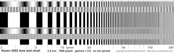
In this page we discuss lens testing (actually, testing complete photographic systems) using the Koren 2003 lens test chart, which has continuously varying spatial frequency. You can download, print and assemble it yourself. This approach is primarily intended for film images, but Imatest Log frequency analyzes digitized images of the chart described below.
For digital cameras or digitized film images, the approach used by Imatest is far more accurate and convenient.
| Green is for geeks. Do you get excited by a good equation? Were you passionate about your college math classes? Then you're probably a math geek— a member of a maligned and misunderstood but highly elite fellowship. The text in green is for you. If you're normal or mathematically challenged, you may skip these sections. You'll never know what you missed. |
| Robert Monaghan's Lens Resolution Testing page contains links to test targets and serious discussions about image sharpness. His Medium Format Articles Page is also a great resource. | |||
| Bob Atkins, the busy director of the photo.net nature photography pages, had a page on Technical Optics that covers lens testing. He also sells a lens test kit based on a modified USAF 1951 test chart. | |||
| Richard Stringer, a Canadian cinematographer, has developed a set of Target Resolution Charts for use in the film industry. A significant improvement over USAF 1951. | |||
|
|||
| Lens testing charts from Sine Patterns, LLC Specialized industrial strength targets. | |||
| How to test a lens by Charles Sleicher, PhD, is full of valuable tips. Excellent reading. He also sells a test kit derived from the USAF 1951 chart. | |||
| PDML lens testing procedure Uses USAF chart. | |||
| ZGC Motion Picture Film & Video Sales and Service has several charts. Their 7A9 Sharpness Indicator Test Chart is quite interesting. | |||
| Photodo articles on MTF and lens performance Extremely informative, but little detail on their testing techniques, which use elaborate equipment not available to consumers. Photodo also has a large data base of lens tests. They stopped testing lenses in 2000 because of a familiar Internet problem: no money to be made. | |||
| Ken Rockwell's glossary of lens testing terms A reminder that there's more to lens quality than sharpness. | |||
| Resolution test patterns Page by John Beale. Contains a nice Postscript/PDF test pattern. | |||
| Horst Kretzschmar ( www.eos-d60.de ) has started a series of lens tests on the Canon EOS D60 using my lens test charts. The test method is in the article, Machen Sie mit beim neuen Objektivtest an Ihrer Canon EOS-D60. My Deutsch isn't good enough to decipher it; for that I used the Google translator. | |||
| White Paper: Using a Nyquist Chart from Photobit Technology. Good reading on a test chart specific to digital cameras, which can suffer from serious aliasing and Moiré effects. | |||
| William
Castleman has some interesting descriptions of Canon lenses and
bodies,
including the EOS-1Ds
and EOS-1D
Mark II. His latest tests use my Koren
2003 test chart. |
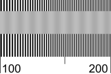
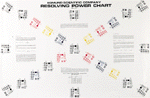
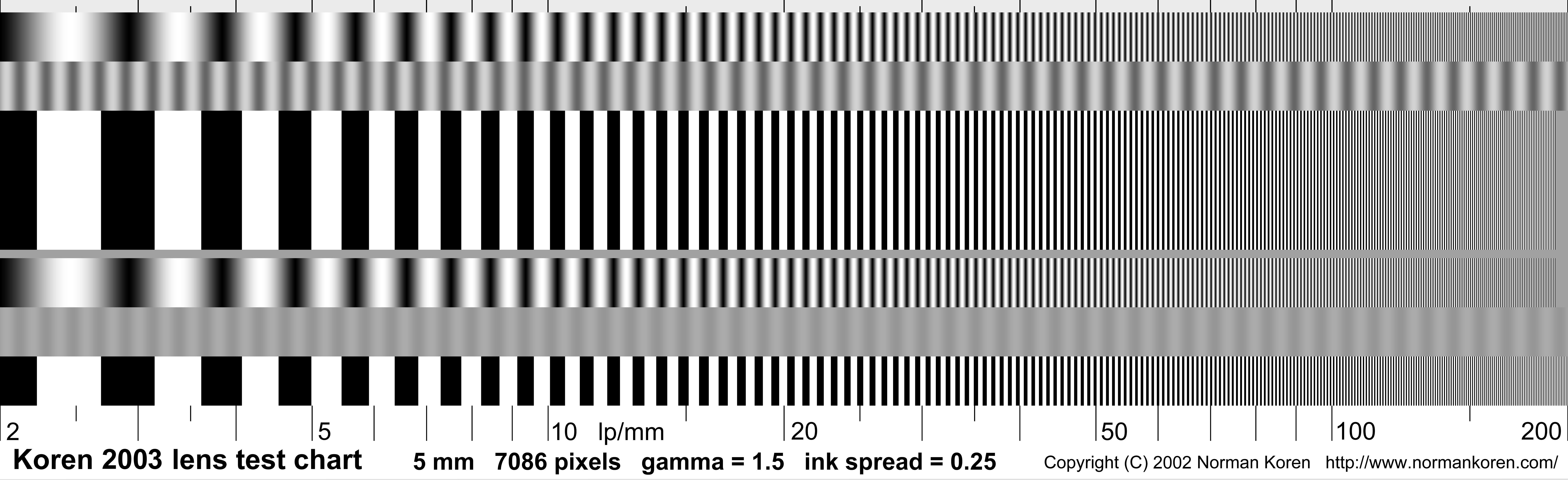
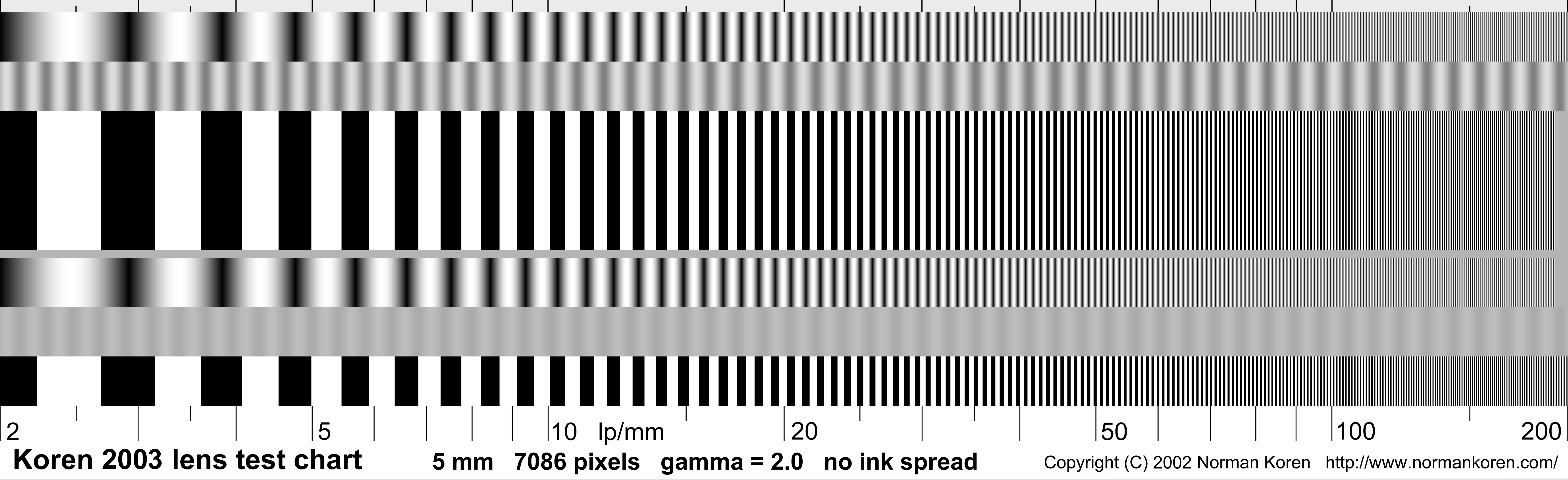
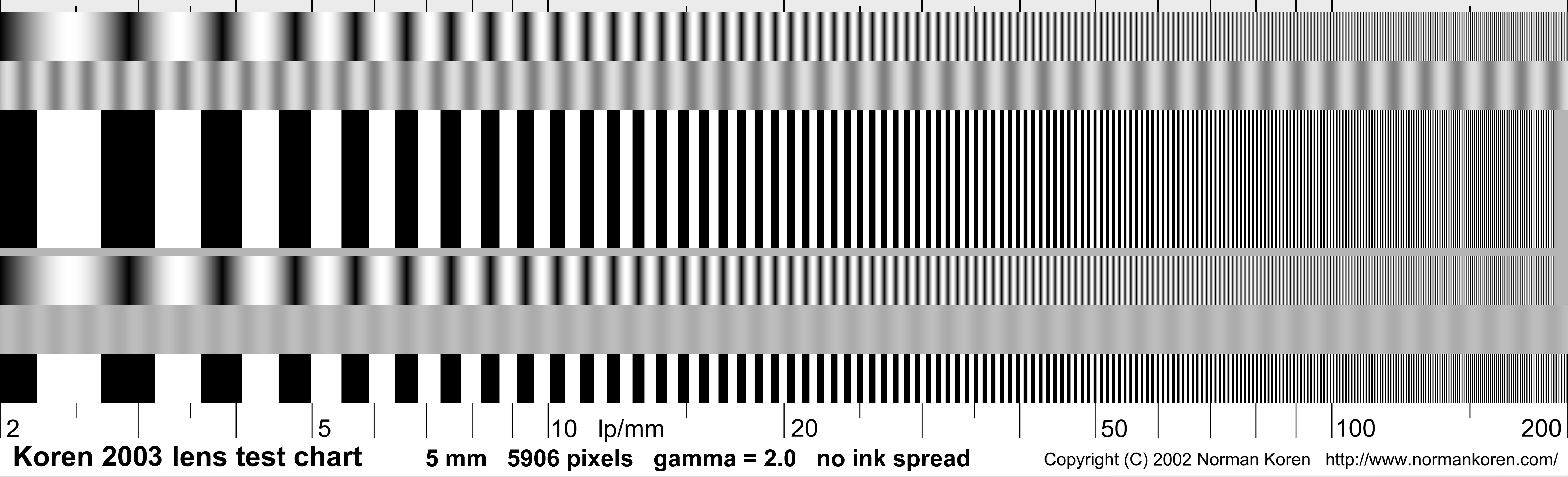
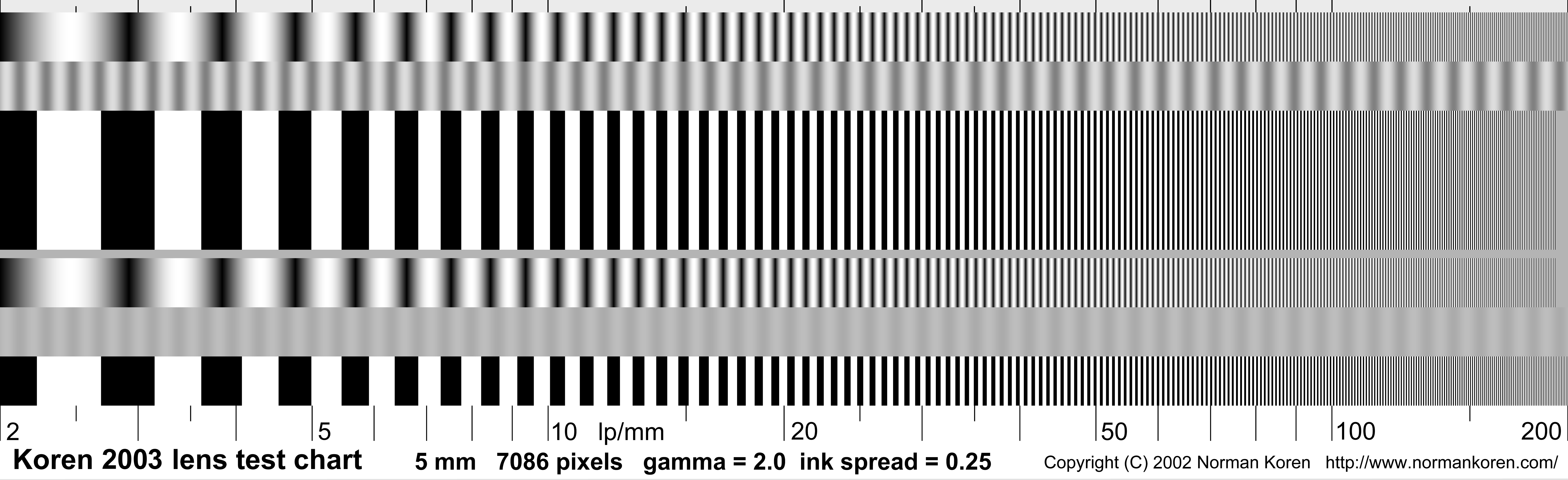
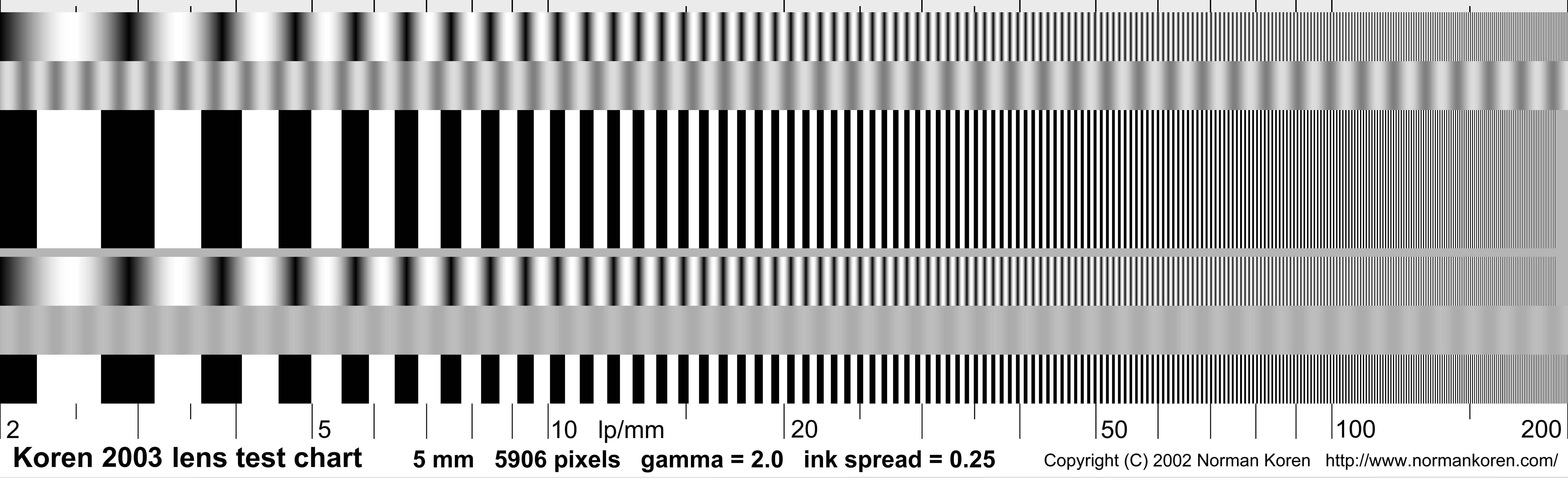
| The USAF 1951 lens test chart (on the right; Robert Monaghan's detailed printable PDF version) and its variants have been a standard for half a century. But it is unsuited for computer analysis because of its fragmented arrangement, and it is poorly suited for visually estimating MTF (Modulation Transfer Function, which is synonymous with spatial frequency response; see Understanding image sharpness part 1). It is often misused. People strain their eyes to find highest resolution at which bars can be distinguished. This frequently results in impressive resolution numbers (over 100 lp/mm) that are poorly related to visible image quality. The goal of testing with the new chart is to be able to say, "at a given f-stop, the center or corner of this lens has 50% MTF at roughly x lp/mm and 10% MTF at y lp/mm. These numbers are well standardized and closely related to perceived image quality and resolution. In this context, MTF means contrast compared to low spatial frequency images. |  |
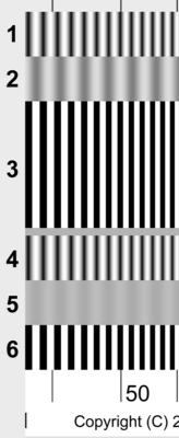 |
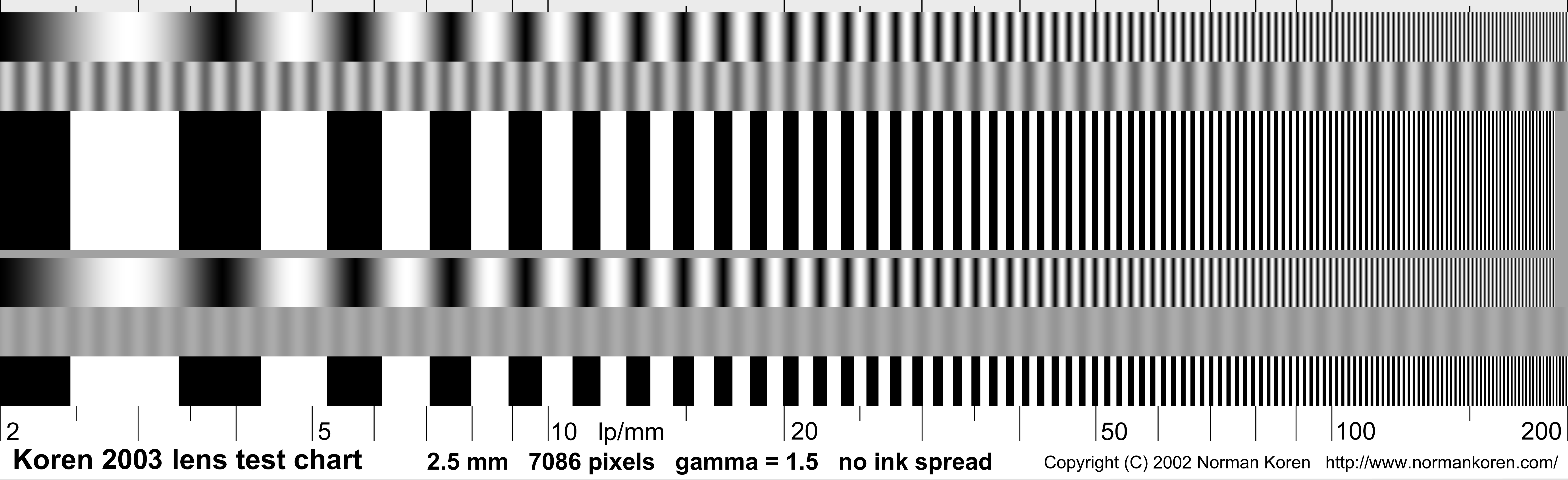
1, 4. Sine pattern, 2-200 lp/mm, for determining MTF
response—
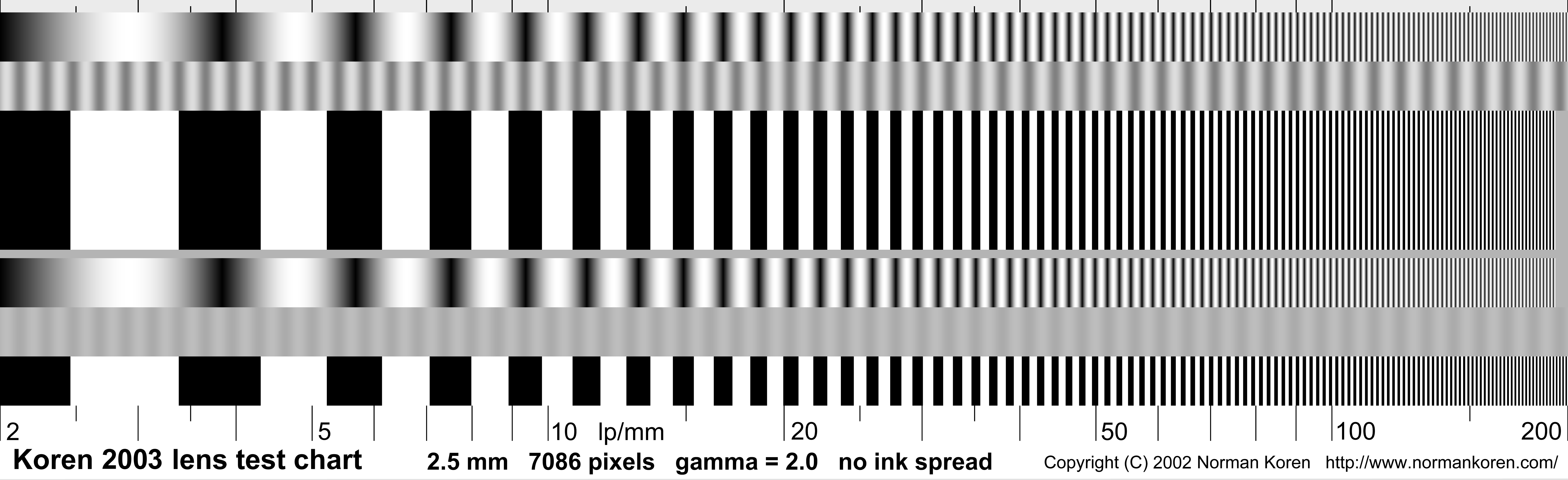
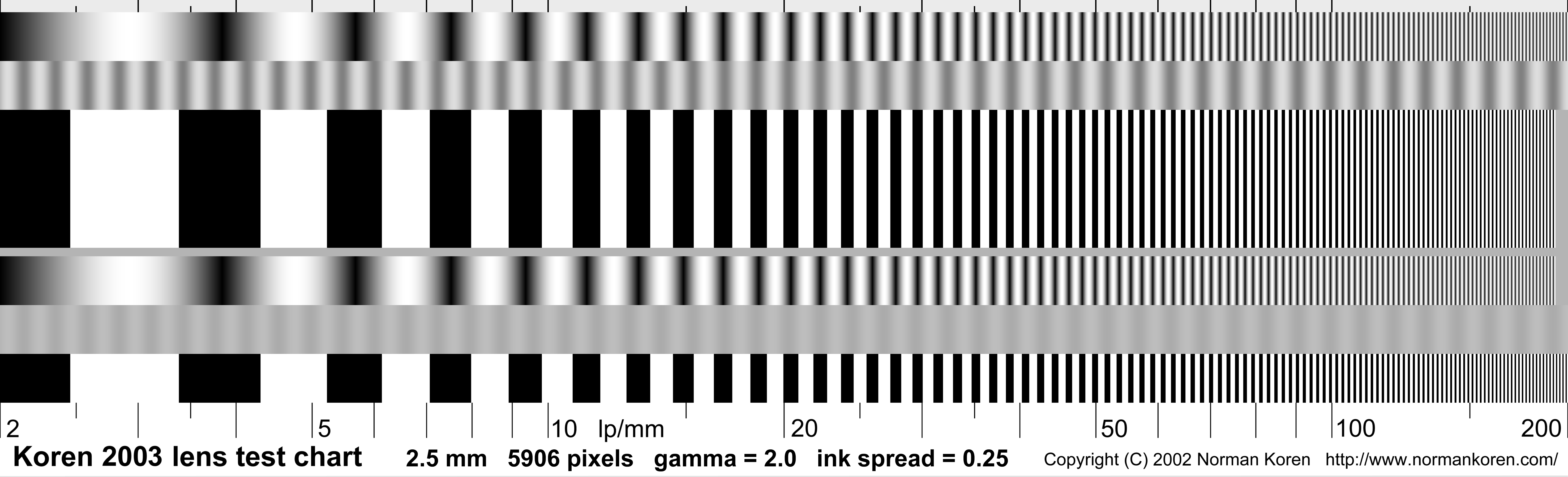
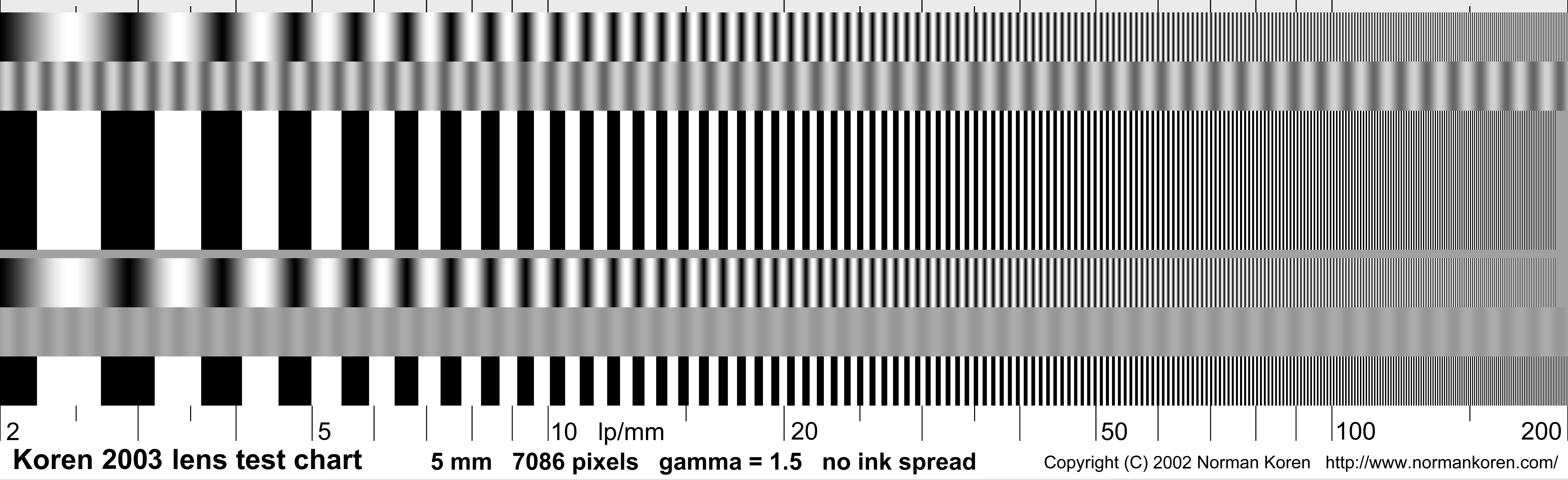
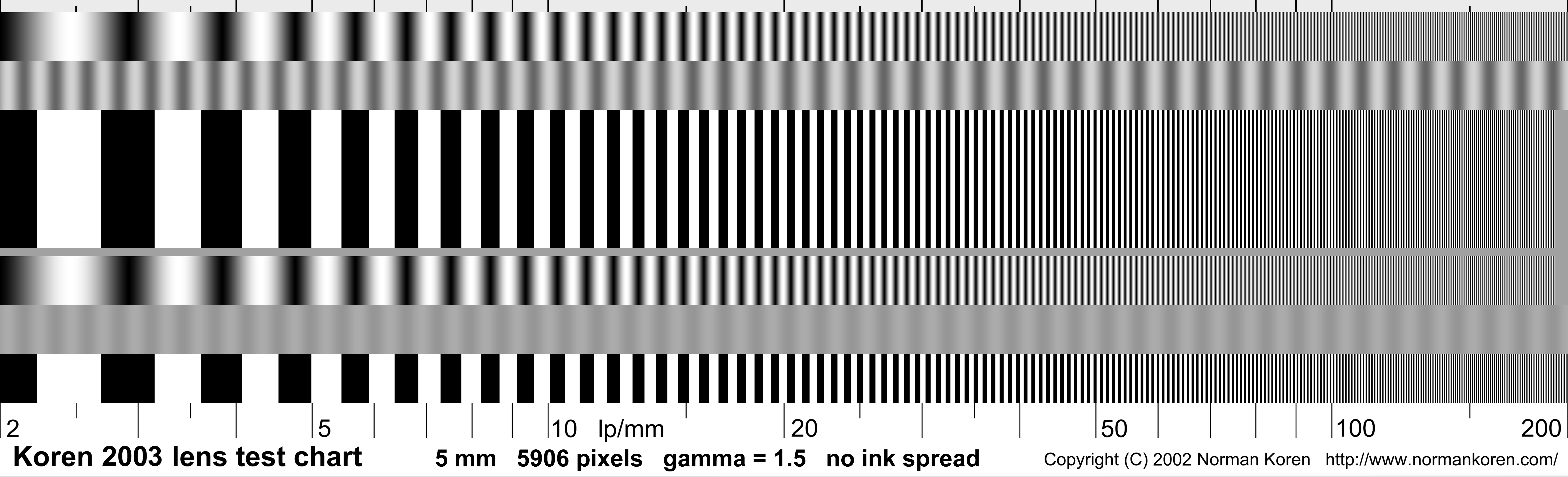
the contrast at a given frequency relative to low frequencies. . 3, 6. Bar pattern, 2-200 lp/m, for observing sharpness— more visible than for the sine pattern. At high spatial frequencies where contrast has dropped by half or more, the bar pattern contrast is higher than the sine pattern by about 27% (a factor of 4/pi). The sine pattern gives correct MTF. . 2. 50% contrast reference: a sine pattern varying between 25 and 75% reflectance at constant spatial frequency. The actual printed level is affected by gamma, discussed below. A sine pattern is used because the image on film appears to be sinusoidal at spatial frequencies where MTF is 50% or less. This band is intended to illustrate the appearance 50% contrast in order to facilitate your visual estimate of the 50% contrast MTF frequency in bands 1 and 4. You should be able to estimate this frequency with an accuracy of around 10%. . 5. 10% contrast reference: a sine pattern varying between 45 and 55% reflectance at constant spatial frequency. Similar to band 2, but intended to illustrate the appearance of 10% contrast. The chart is designed so that each contrast reference band is adjacent to both sine and bar patterns. Contrast reference bands 2 and 5 are not used with digitized images. In addition, there is a thin middle gray reference band between and to the right of bands 3 and 4. |
Chart length: The names of the charts below (2.5 and 5mm) are the intended lengths of the chart when reproduced on film or a digital sensor. They are designed to be printed at 50, 80, or 100x magnification (relative to the intended size on the film or sensor) to avoid printer limitations.
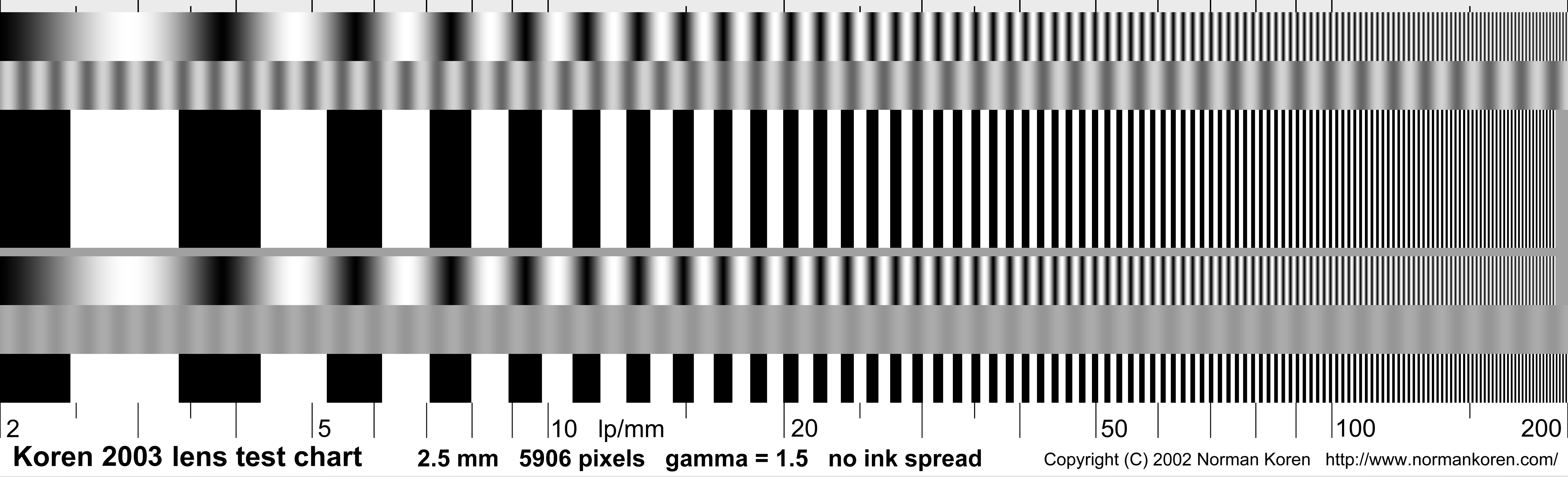
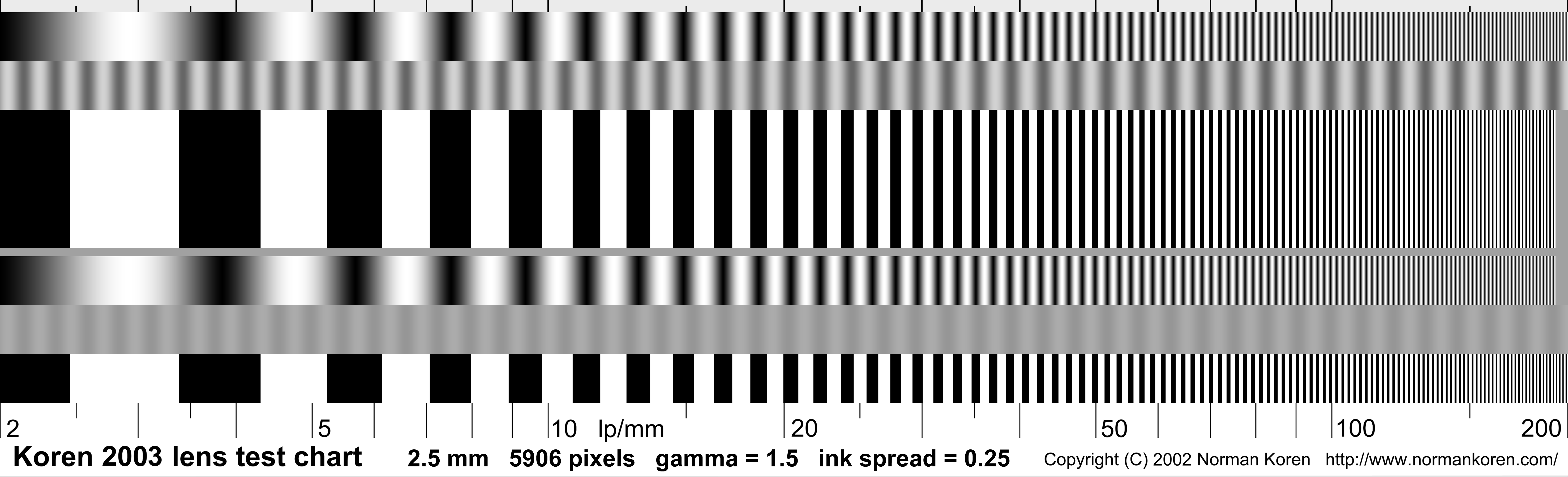
2.5 mm charts (illustrated above) are designed to be printed 25 cm (9.84 inches) long (100x magnification) on a 4.5x11 inch strip— half of a letter sized or A4 sheet. The 7086 pixel long charts are best for printing at multiples of 720 dpi (Epson printers). The 5906 pixel long charts are best for printing at multiples of 600 dpi (Canon and HP printers). 2.5 mm charts are recommended for compact digital cameras, which have tiny sensors (11 mm diagonal or less) and lenses with relatively short focal length.You can print these charts any size you want as long as you note the magnification and photograph them at the appropriate distance, but I recommend the standard sizes to avoid confusion.5 mm charts are designed to be printed 25 cm (9.84 inches) long (50x magnification), which fits on a 4.25x11 inch strip— half of a letter sized or A4 sheet, or 40 cm (15.75 inches) long (80x magnification), which fits on half of an A3 sheet.
Print magnification: advantages/disadvantages
For 24/8-bit image files where pixel levels vary between 0 and 255, if print reflectance varies between 0 (pure black) and 1 (pure white) (it's actually more like 0.01 and 0.95), the simplified equation for print reflectance is,
reflectance = (pixel level/255)gammaFor properly calibrated Windows systems (and sRGB and Adobe RGB color spaces), gamma is 2.2. For older Macintosh systems, gamma is 1.8 (I believe 2.2 is now the standard). Small differences in gamma are barely visible. The Epson 1270 and 2200 printer allows you to select gamma of 1.5, 1.8 or 2.2.
At high spatial frequencies, where the MTF of lenses, film, and sensors is declining, an ideal black and white bar pattern (1) gradually merges into 50% gray (halfway between black and white). The actual gray level is affected by ink spread (dot gain) in the printed chart. The average reflectivity of the reference patterns depends on printer gamma. To facilitate visual comparison, it should be close to the gray level of the merged bar pattern. Because many variables affect this match, two sets of charts are available, illustrated below.
 |
 |
|
|
|
The charts are written so that 50% gray has a normalized pixel level (pixel value/255) of 0.51/gamma (0.707 for gamma = 2). When they are printed at the specified gamma (2 is close enough to 1.8 or 2.2), 50% gray should be printed at the correct level. But because reality can be a bit messy— the actual levels are affected by ink spread, printer drivers, and other factors, the gamma = 1.5 chart may look better printed. If needs be, you can adjust gamma in your image editor by using a gamma or curvesFor best accuracy, you may want to adjust gamma in the digitized result to minimize gamma distortion, which is plainly visible in the readback charts below, where the sine waves are somewhat rounded on top and sharp on the bottom (dot gain distortion is also present). I find that a modest amount of gamma distortion doesn't degrade the results severely.
Pixel length: The 7086 pixel (length) charts are best for printing 25 cm (9.8425 inch) long charts with printers that operate at multiples of 720 dpi (Epson). At least 1440 dpi is recommended. The 5906x1798 pixel charts are best for printing 25 cm long charts with printers that operate at multiples of 600 dpi (Canon and HP). At least 1200 dpi is recommended.
Ink spread (also called dot gain), present in most inkjet printers, affects the printed appearance of the bar pattern at the highest spatial frequencies. The overall tonal effects of ink spreading is compensated in software (by ICC profiles, etc.), but fine line patterns can't be compensated. In charts with ink spread = 0, black and white bars have the same width; they aren't compensated for ink spread. In charts with inkspread = 0.25, black bars are narrowed by a fixed amount, equal to a factor of 0.25 at the highest spatial frequency.
| Chart
length on film or sensor (note 1) |
Gamma (note 3) |
Ink spread (note 4) |
Pixel length (note 5) |
File name |
| 2.5 mm
M = 100 |
1.5 | 0 | 7086 5906 |
Lenstarg_25_7086p_15g_0is.png
Lenstarg_25_5906p_15g_0is.png |
| 1.5 | 0.25 | 7086 5906 |
Lenstarg_25_7086p_15g_25is.png
Lenstarg_25_5906p_15g_25is.png |
|
| 2 | 0 | 7086 5906 |
Lenstarg_25_7086p_20g_0is.png
Lenstarg_25_5906p_20g_0is.png |
|
| 2 | 0.25 | 7086 5906 |
Lenstarg_25_7086p_20g_25is.png
Lenstarg_25_5906p_20g_25is.png |
|
| 5 mm
M = 50 |
1.5 | 0 | 7086 5906 |
Lenstarg_50_7086p_15g_0is.png
Lenstarg_50_5906p_15g_0is.png |
| 1.5 | 0.25 | 7086 5906 |
Lenstarg_50_7086p_15g_25is.png
Lenstarg_50_5906p_15g_25is.png |
|
| 2 | 0 | 7086 5906 |
Lenstarg_50_7086p_20g_0is.png
Lenstarg_50_5906p_20g_0is.png |
|
| 2 | 0.25 | 7086 5906 |
Lenstarg_50_7086p_20g_25is.png
Lenstarg_50_5906p_20g_25is.png |
Notes
Copyright notice: All lens test charts are copyright © 2001-2003 by Norman Koren. These charts may be reproduced without restriction for personal use. Permission is granted to publish test results using these charts providing you credit the author, including a link to this web page (if it's published on the Internet). Please inform the author via e-mail. Contact me if you are interested in publishing these charts with a high quality process that would allow the use of lower magnification.
 You
will need to open the chart in your image editor and print several
copies
with you printer set to its highest resolution. Use glossy, semigloss,
or luster paper for best detail. You may want to slit standard sheets
of
paper lengthwise: two 4.25x11 inch strips from an 8.5x11
sheet, etc. Check to make sure the average density of the gray tones in
the 10%
contrast reference band (5) is close to the average density at high
spatial
frequencies for the bar and sine patterns (viewed from a distance). You
may have to make a
curves
or gamma adjustment if it isn't. I
recommend
examining the printed chart under a loupe (at least 10x)
to be sure the sine and bar patterns are clear at high spatial
frequencies.
You
will need to open the chart in your image editor and print several
copies
with you printer set to its highest resolution. Use glossy, semigloss,
or luster paper for best detail. You may want to slit standard sheets
of
paper lengthwise: two 4.25x11 inch strips from an 8.5x11
sheet, etc. Check to make sure the average density of the gray tones in
the 10%
contrast reference band (5) is close to the average density at high
spatial
frequencies for the bar and sine patterns (viewed from a distance). You
may have to make a
curves
or gamma adjustment if it isn't. I
recommend
examining the printed chart under a loupe (at least 10x)
to be sure the sine and bar patterns are clear at high spatial
frequencies.
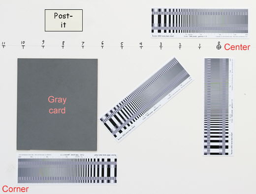
Next, assemble the charts into a target. I recommend using 32x40 inch foam board (larger if convenient), which is available at any art supply store. Charts can be safely attached using stick glue. (One widely available brand, Ross Stik, claims to be acid free.) An example of a target, designed for the 22.7x15.1 mm sensor of the Canon EOS-10D, is shown on the right. (The entire target isn't shown— there is more on the left and the bottom to accomodate the 24x36 mm 35mm format.) You may want to take advantage of available real estate and include a gray card and a color chart— you might as well test for lens attributes other than sharpness. Digital Dog's Printer test file, illustrated in Making fine prints in your digital darkroom, would be a good choice. Leave room for a Post-it, which you'll use for critical information (lens, focal length, f-stop). This isn't necessary with a modern digital camera like the EOS-10D, which records it all. You may also want to add some charts at an angle.
 Draw
a scale on the target to
represent
the distance from the center of the sensor in 1 mm increments. For the
target in the illustration, which uses 5 cm charts intended for 50x
magnification, the 1 mm marks were placed every 5 cm. The center of the
target in the photograph (easy to locate in the viewfinder) is placed
just
below the number 0 on the scale, near the upper right of the target.
Draw
a scale on the target to
represent
the distance from the center of the sensor in 1 mm increments. For the
target in the illustration, which uses 5 cm charts intended for 50x
magnification, the 1 mm marks were placed every 5 cm. The center of the
target in the photograph (easy to locate in the viewfinder) is placed
just
below the number 0 on the scale, near the upper right of the target.
The scale is useful for setting camera-to-target distance. Since the distance from the center to the edge of the EOS-10D sensor is 22.7/2 = 11.35 mm, the left side of the image should be aligned with 11.3 on the scale. You would use 18 mm for a 24x36 mm frame with 35mm film. Since most viewfinders show less than the full image I aligned it at just under 11 to get close to 11.3. This technique is a lot easier than using a tape measure. With a little trial-and-error (and a tape measure for calibration) you'll get it just right.
d1+d2 = film-to-target distance = (M+2) f ..(close approximation for M>>1)Use M = 50 or 100, as indicated above. A measuring tape is more accurate than the distance scale on most lenses (particularly 35mm zooms), which indicates d1+d2. The easiest way to set distance is with a scale on the target, as described above.
Derivation The simplified lens
equation is
1/d1 + 1/d2 = 1/f whered1 is the lens-to-object distance (target for those of us who aren't optics geeks); d2 is the lens-to-film distance; f is the lens's focal length. The magnification (in this case, magnification of the object (the printed target) with respect to image on the film) is. M = d1/d2Using 1/d2 = M/d1, we can solve for d1: 1/d1 + M/d1 = 1/f = (1 + M)/d1 ; d1 = (M+1) f . |
Example— Suppose
you are testing a 200 mm telephoto lens. With the 5 mm targets the
nominal
magnification (the magnification where the lp/mm scale reads correctly)
is 50. The lens-to-target distance is d1 =(M+1)
f
= 51*200 mm = 10.2 meters = 401.6 inches = 33.46
feet.
That's quite large— impractical for most indoor locations. (Don't even
think of using a 2.5 mm target, which has M = 100, for long
lenses.)
You may want to use half the nominal magnification for this target: M
= 25. If you do this the actual lp/mm reading will be
half the reading
on the chart, i.e., the maximum lp/mm becomes 100 instead of 200.
That's
sufficient in most realistic cases. d1
=(M+1)
f = 26*200 mm = 5.2 meters
= 204.7 inches = 17.06 feet. Better.
.
Other
distances
and magnifications You may not know the
precise
focal length of the lens (zooms are often poorly marked), or you may
find
distance
d1 to be inconvenient, especially for long lenses
(large
f ). You may want to use a magnification Mactual
lower than the nominal magnification M (50 or 100), for
example,
Mactual
= M/2. In these cases you can apply a correction
factor to the lp/mm spatial frequency. This isn't
difficult
in practice, particularly for digital cameras or scanned images, where
you should know the pixel spacing.
The key is to measure a length on the film or digital sensor and
compare
it with a specified length. The actual lp/mm is
lp/mm (actual) = (lp/mm on chart) * (specified length) / (measured length)
Length can refer to the chart or the entire target. If you are working with a digitized image, measured chart length is easy to find: it's the pixel spacing times the chart length in pixels. Specified chart length (2.5 or 5 mm) is given in the above table. For example, suppose the measured chart length for a 5 mm chart is 7.7 mm. The actual lp/mm would be 5/7.7 = 0.649 times the lp/mm indicated on the chart.
You can also use the scale on the target. If you place "0" at the center of the image, measured length is the value of the scale at the edge of the image. Specified length is half the width of the image sensor or frame, for example, 11.35 mm for the 22.7x15.1 mm sensor of the Canon EOS-10D or 18 mm for a 36x24mm frame on 35mm film.
Note that with Imatest Log frequency, distance is not critical because spatial frequencies are automatically detected.
 You
can evaluate the results by observing film visually or scanning it
(more
accurate, but spatial frequencies will be limited by the scanner). Skip
to Interpreting digitized results if you are
using
a digital image.
You
can evaluate the results by observing film visually or scanning it
(more
accurate, but spatial frequencies will be limited by the scanner). Skip
to Interpreting digitized results if you are
using
a digital image.
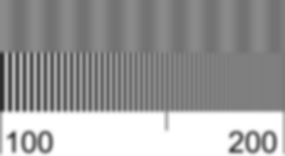
| Here is an example of how to use the chart— not
a real lens test. The chart on the right has been
softened
using gaussian blur. Look for the frequency where the sine pattern
contrast
is similar to the contrast of the 50% or 10% contrast reference bands
(2
and 5, above). The illustration on the right
includes
portions of the pattern and the 10% contrast band. The 10% MTF
frequency
is approximately 150 lp/mm. It is difficult to estimate this frequency
with accuracy better than about ±15% because MTF rolls off
slowly
for gaussian blur.
MTF rolls off more rapidly for actual lenses; hence a better estimate of the 10% (and 50%) MTF frequency should be possible. |
 |
Whichever approach you choose, you'll want to compare the primary sine pattern, band 1 or 4, with the 50% and 10% contrast reference bands, 2 and 5, to determine the spatial frequency (lp/mm) for the corresponding MTF.
Remember that a number of factors can degrade the results: poor film flatness, camera shake, sloppy film development and focus error among them. When I obtained my Hasselblad 500C, the ground glass focusing screen was out of adjustment. I had to adjust it a jeweler's screwdriver using an image at infinity. Remember also that sharpness may be dominated by the film. According to Zeiss (Camera Lens News No. 10 article on film flatness), "more than 99% of all customer complaints about lacking sharpness in their photos can be attributed to misalignments of critical components in camera, viewfinder, or magazine, focus errors, camera shake and vibrations, film curvature, and other reasons."
You'll want to compare your test results with calculated results in Parts 1 and 2. Don't expect grandiose numbers, over 100 lp/mm. For Fujichrome Velvia with an excellent lens, the 50% and 10% MTF frequencies (f50 and f10) are 37 and 67 lp/mm— limited mostly by the film. 4000 dpi scanning drops these numbers 10 to 15%, but you can recover a lot— actually achieve better f50 than the unscanned image— by sharpening. You'll learn to appreciate careful technique. Images that actually achieve this sharpness can be quite impressive: I've frequently fooled people into thinking I was using the next larger format.
|
 Although the most accurate and convenient way to analyze digitized images is with Imatest Log frequency, there are some free alternatives.
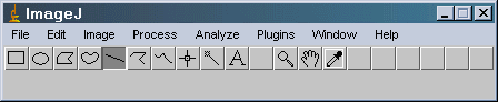
ImageJ is a standalone public domain image analysis program, written in Java. You can learn about ImageJ in the Documentation (the Plot Profile command is of particular interest), and download the appropriate version (Macintosh, Windows, Linux, etc.) by clicking here. Installation is utter simplicity— just unzip the file and copy the ImageJ shortcut to a convenient location. Double-click (in Windows) to run. The screen on the right comes up.
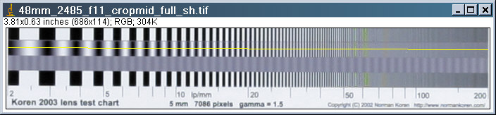
Open the scanned or digital camera image, with File, Open. Select the line tool (shown) and use the mouse to draw a line along the portion of the image you wish to analyze. You should know the spatial frequency at the start and end of the line. Here is an example, using a cropped image— cropping is preferable but not necessary. You can draw the line wherever you like. Note that the spatial frequency increases logarithmically (2 to 200 lp/mm (or other arbitrary units) in this illustration).
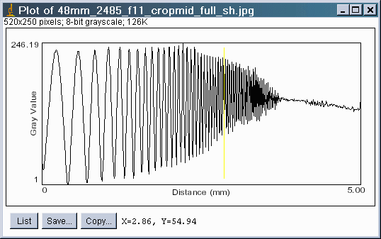
After you've drawn the line, click on Analyze, Set Scale... The nonzero Distance in Pixels: (length) of the line should be shown. Set Known Distance: to 1 (or 100 if you like percent) or to a known length (I chose 5 mm for the target). Unit of Length: can be anything as long as it's not blank. Click OK. Then click Analyze, Plot Profile. The window below appears. Pretty cool.
 Spatial
frequency vs. normalized distance
Spatial
frequency vs. normalized distance
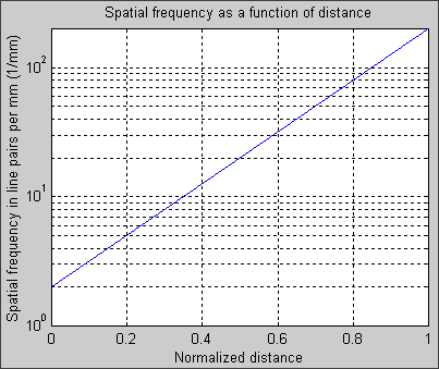
On my charts, frequency increases logarithmically. Let f1 be the lowest spatial frequency, on the left of the chart, corresponding to X* = X/Xmax = 0. Let f2 be the highest spatial frequency, on the right of the chart, corresponding to X* = 1. The spatial frequency f at X* is,
f = f1 ( f2 / f1 )X* ; Using ax = exp(x ln(a)), we calculate the inverse,In this example, the approximate 50% MTF frequency corresponds to the vertical yellow line (which I added in ImageJ) at X* = 0.572. This is a rough guess— perhaps high— because of gamma and dot gain distortion. For f1 = 2 lp/mm and f2 = 200 lp/mm, f50 = 2(100)0.572 = 27.9 lp/mm. The approximate 10% MTF is approximately X = 3.50; X* = 0.7. f10= 2(100)0.70 = 50.2 lp/mm. (For reference, the Nyquist frequency for the EOS-10D is 67.6 lp/mm.) This is close to the estimates from DPreview.com's EOS-D60 review (which used the superb 50mm f/1.4 stopped down to f/9). The 10% MTF scale number, which is close to the absolute cutoff, is about 17. Using the technique described elsewhere, this is 17*50/15.1 = 56 lp/mm. List shows the values of the plot and Save saves an ASCII file with (point value) on each line. This file can be used by separate programs such as Excel for further analysis.
X* = ln( f / f1 ) / ln( f2 / f1 )
PixelProfile is another simple program that can generate a plot of pixel values along a line. It's simpler to use and less versatile than ImageJ. It also outputs data points in Excel format. You can choose between plots of R, G, B, H, S, V, or Intensity. Image size is limited to 640x480 pixels. (Thanks to Chuck Varney, I discovered it in late March 2003.) I'm also exploring Dataplot, a free public domain scientific/visualization software package from NIST, and GNU Octave, both of which could be useful for analysis.
The PixelProfile plot is nice because it has grid lines, which make it easier to interpret the data. Because of the 640 pixel horizontal limit it doesn't plot the entire chart, but it goes far enough in this case. The X-scale is in pixels. To calculate spatial frequency f from the above equation, you'll need to calculate X* = X/Xmax, where Xmax is the length of the pattern in pixels. The best way to find Xmax is with an external editor. Xmax = 682 pixels for this chart.
| VB | The average luminance for black areas— at low spatial frequencies. |
| VW | The average luminance for white areas— at low spatial frequencies. |
| Vmin | The minimum luminance for a pattern near a given frequency or scale value (a "valley" or "negative peak"). |
| Vmax | The maximum luminance for a pattern near a given frequency or scale value (a "peak"). |
Use the following equations to find MTF.
| C(0) = (VW-VB)/(VW+VB) is the low frequency (black-white) contrast. |
| C(f) = (Vmax-Vmin)/(Vmax+Vmin) is the contrast at spatial frequency f. Normalizing contrast in this way— dividing by Vmax+Vmin (VW+VB at low spatial frequencies)— minimizes errors due to nonlinearities in acquiring the pattern. |
| MTF(f) = 100%*C(f)/C(0), for the sine pattern. Valid at all frequencies. |
| MTF(f) ~= 78.5%*C(f)/C(0), for the bar pattern, valid where C(f) < 0.7*C(0) The 78.5% factor is explained in the box below. |
Example: Use the above PixelProfile plot to find MTF at 40 lp/mm (a spatial frequency often used in lens test charts). X* = ln(40/2)/ln(200/2) = 0.650. Since Xmax = 682 pixels, X = X* Xmax = 444 pixels. At this frequency, the envelope average is Vmin = 112 and Vmax = 198. C(40 lp/mm) = (198-112)/(198+112) = 0.277. At low frequencies, VB = 4 and VW = 234. C(0) = (234-4)/(234+4) = 0.966. MTF(40 lp/mm) = 0.410/0.966 = 0.287 = 28.7%. The excellent lens (the Canon 28-70 f/2.8 L) has MTF of about 70% at this frequency at the center. The 24-85 consumer zoom is quite good at f/5.6-f/11, but probably not quite as good as the 28-70 L. The remainder of the MTF loss is due to the sensor. The hand method is tedious and not as accurate as I'd like. So I developed something better.
sfrcalc .A Matlab program for calculating spatial frequency response (equivalent to MTF)
|
Thanks
to Chuck
Varney for
prodding
me into this.
.
I wrote sfrcalc, in Matlab, which is required to run it. I used Matlab because it's familiar. Ideally I'd like to make it standalone— perhaps as an ImageJ plugin, but the learning curve looks pretty serious. If anyone wants to try, the math is pretty simple. I use the equation for MTF(f) above. Most of the code is for the output. You can download sfrcalc by right-clicking here. Sfrcalc displays spatial frequency response (SFR), which is essentially the same thing as MTF. SFR usually refers to a complete photographic system while MTF refers to individual components. I often use them interchangeably. To run sfrcalc,
sfrcalc file.txt s1 s2 ph —where— file.txt is the input file name. s1 is the minimum scale value in lp/mm. s2 is the maximum scale value in lp/mm. ph is the picture height in mm (15.1 for the 10D, 24 for 35mm). Example: sfrcalc EOS2485.dat 2 80 15.1 |
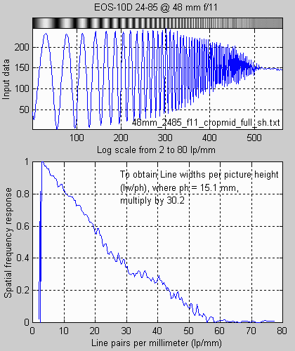 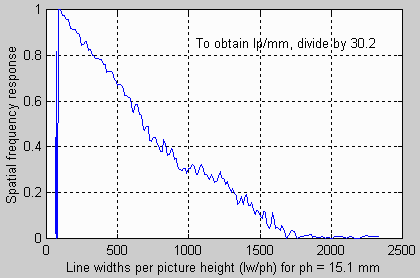 |
The little bumps on the SFR plots aren't real. They're the result of sampling phase errors (significant in the 10D), grain (or noise; very low in the 10D), and imprefections in the printed chart. They aren't systematic— they average out. The true MTF would be a line that smooths them.
The upper SFR plot uses Line pairs per mm
(lp/mm)
on the horizontal axis. The lower SFR plot (with the top part cropped
out)
uses Line widths per picture height (lw/ph, where there are 2 line widths
per line pair). This plot is valuable for comparing cameras
with
different formats (i.e., digital vs. 35mm), but with similar aspect
ratios.
See my EOS-10D
page.
For this lens, which I characterize as "pretty good" (it's not an
L-series
lens), the 50% MTF frequency (f50, closely related to perceived image
sharpness)
is about 22 lp/mm, or 700 lw/ph. The 10% MTF frequency (f10; closely
related
to traditional resolution measurements) is 49 lp/mm, or 1500 lw/ph.
Note
that 1000 lw/ph is equivalent to 10 on the Dpreview.com
charts.
.
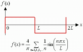 Approximating
MTF from bar patterns Approximating
MTF from bar patterns (the pi/4 discrepancy) MTF is based on sine wave response, but we often work with bar charts. The contrast ratio obtained directly from a bar chart is called the contrast transfer function, CTF( f ) = 100% * C( f ) / C(0). CTF is rarely referred to in the literature. It is not the same as MTF. A portion of a bar chart can be approximated by a periodic function called a square wave, illustrated above for period 2L (frequency = f = 1/2L). Fourier transform mathematics teaches us that any periodic function can be expressed as an infinite sum of sine functions, starting with the fundamental, sin(pi*x/L) = sin(2*pi*f ), and including harmonics, sin(n*pi*x/L) = sin(2*n*pi*f ) for n = 2, 3, 4, ... The equation for the square wave is shown above. It only has odd harmonics (n = 3, 5, 7,...). The amplitude of the fundamental frequency of the bar pattern is 4/pi = 1.273 times the amplitude of the bar pattern itself. To obtain MTF from CTF you must multiply by a factor of pi/4, hence, MTF( f ) = 0.785*CTF ~= 78.5%*C(f)/C(0), where C(f) < 0.7*C(0)This equation is only accurate at relatively high frequencies where response is dropping— where the harmonics are strongly attenuated. These are the frequencies of interest. The exact equation for
relating
MTF( f ) to CTF( f ) was given by Coltman (1954):
|

| Images and text copyright © 2000-2013 by Norman Koren. Norman Koren lives in Boulder, Colorado, where he worked in developing magnetic recording technology for high capacity data storage systems until 2001. Since 2003 most of his time has been devoted to the development of Imatest. He has been involved with photography since 1964. |  |
