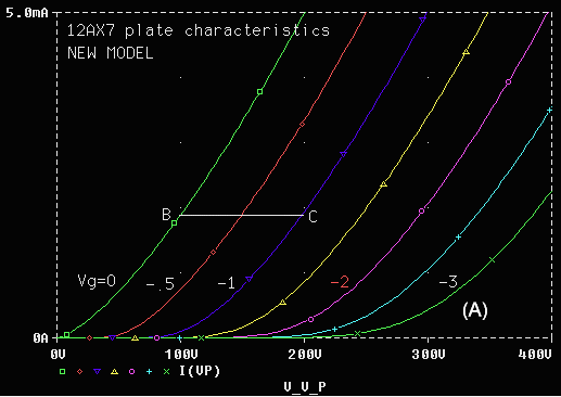
Figure 2. 12AX7 plate curve from the new model.
Finding SPICE tube model parametersby Norman L. Koren
Released August 24, 2001; updated Jan. 5, 2008 This article presents a Matlab program for finding parameters for SPICE tube models-- a great savings in time and tedium over the trial-and-error method in Improved vacuum tube models for SPICE simulations.
James E. Lanier's PSPICE Triode Calculator is a promising program for finding tube model parameters. It's still under development; he plans to expand it to include tetrodes and pentodes. Jeroen's Technical Center: Motega (Modeling Of Tubes Employing Genetic Algorithms). Another promising program for finding tube model parameters. Written in Matlab. |
In 1998 I wrote Tuparam, a Matlab program for finding the parameters using nonlinear optimization. My Matlab skills at the time weren't adequate to accomplish everything I wanted, so I set it aside. My skills have improved considerably since then.
Matlab is a popular program with engineers, though it's not as widely available as programs like Excel. Unlike PSpice, there is no free evaluation version. But the student version is relatively inexpensive. If you intend to use Tuparam you should be reasonably familiar with using Matlab and reading m-files (Matlab programs). You don't need to be an expert. Matlab versions are notoriously incompatible. I developed the program on versions 5.1 and 5.3. You may need to tinker with the program to get it to run on other versions. On earlier versions you may need to change the solver from the fminsearch to the fmins. Instructions are in the m-file. Consider the program a beta version. I haven't debugged it as thoroughly as I might if it were a commercial product. But it's free.
Since I wrote the program I've discovered the work of two other people who've approached the problem.
E1 = (EP
/kP)
log(1 + exp(kP(1/µ
+
EG
/sqrt(kVB
+
EP2))))
IP = (E1X/kG1)(1
+ sgn(E1))
The new plate current equation for pentodes is similar to that of triodes:
E1
= (EG2 /kP)
log(1 + exp(kP (1/µ+EG
/EG2)))
IP = (E1X/kG1)(1
+ sgn(E1)) arctan(EP
/kVB)
IP = (EG+EG2
/µ)3/2/kG2
for EG+EG2
/µ
>= 0
= 0 otherwise.
The parameters required to describe tube performance are µ, X, kG1, kG2, kP, and kVB . kG2 is for pentodes only. The purpose of the Tuparam program (and of this entire page) is to find them. Plate curves for the 12AX7 with manually-derived parameters are shown below.
Figure 2. 12AX7 plate curve from the new model.
To run Tuparam from the Matlab window, enter,
cd dirctory_pathwhere dirctory_path is the full pathname of the directory that contains the Tuparam program and data files. filename is a Matlab m-file that contains raw data derived from charts, written as Matlab assignment statements. Several examples are included. It may also contain initial parameter guesses (which facilitate the optimization) and entries to control the plot. The following table lists most of the input variables. Many are optional, and a few omitted here are mentioned in the program listing.
Tuparam filename
| Parameter | Description |
| Input data from
characteristic curves |
|
| Vp | Plate voltage array. Format : [ Vp(1) Vp(2) ...].
Vp(i) must correspond to Vg(i), Idata (i), and (pentode only) Vs(i). There should be a minimum of 5 entries for triodes and 6 for pentodes. More strongly preferred! |
| Vg | Grid voltage array. |
| Idata | Plate current array. |
| Vs
(Pentode) |
Screen grid voltage array. TubeType is set to 'PENTODE' if Vs is entered; otherwise it's 'TRIODE'.. A single value may be entered, but an array is recommended. The first value must come from the pentode characteristic curve (determines the screen voltage in the pentode output curve). Best results are obtained if several values of Vs are available, as they would from the triode curve. |
| Plot control | |
| TubeName | The name of the tube ('12AX7A', 'EL34', etc.) |
| Source | The source of the data and other relevant notes. Goes into a comment line in the model file. |
| VGP [0:-5:-30] | Grid voltages for plot. Formats: either A:B:C (A to C in steps of B) or array [v1 v2 ...]. |
| VGTRI | Grid voltages for pentode triode-mode plot . Same formats as VGP. |
| Vpmax [450] | Maximum plate voltage for plot. |
| axset
[ automatic ] |
Axis settings for plot: [V(min) V(max) i(min) i(max)] where V is volts displayed on the horizontal axis and i is current (Amperes) displayed on the vertical axis. Set automatically if not entered. Can be adjusted after running Tuparam. |
| Initial guesses
[default] |
(There aren't always necessary to enter, but they can speed up the simulation and facilitate convergence.) Explained in Improved vacuum tube models for SPICE simulations. |
| MU [20] | µ Amplification factor. It helps convergence to have a good guess. |
| KG1 [2000] | kG1 Inversely proportional to overall plate current. |
| EX [1.35] | X Exponent: rarely need to change. Not optimized if only a single value of Vs is entered for Pentodes. |
| KVB [10 for small signal
triode; 40 for pentode] |
kVB Knee volts. A good initial guess helps convergence. |
| KP [60] | kP Affects opration in region of large plate voltage and large negative grid voltage. |
| VCT [0] | Contact potential. An offset voltage on the grid that makes curves appear as if they are going positive on a few older tube types (RCA, Sylvania 12AX7, 12AU7). |
| KG2 [4500] | kG2 Inverse screen grid current sensitivity. NOT OPTIMIZED. The entered value is kept. |
The most important aspect of the input data is the data from the tube curves, in Vp, Vg, Vs (Pentode only) and Idata, below. The points corresponding to these entries are shown as asterisks (*) or circles (O) in the charts below, where * is for Pentode charts and O is for triode charts, including pentode data in triode mode. It is important that data points be scattered around the chart, and that they represent all likely operating conditions and chart features. Only a minimum of 5 is required, but more help the solver converge accurately. Check especially carefully for errors.
For pentodes it is best to have data at more than one screen voltage. I perfer to enter some data from the pentode curves (fixed grid screen voltage) and some from the triode curves (the screen grid and plate connected). The pentode data should be entered first: the first screen voltage is used for the pentode plots.
Tuparam uses the fminsearch solver, which is part of standard Matlab. If you have the Optimization toolbox, you should use the fsolve solver, which works more efficiently and is less dependent on good initial conditions. Instructions for changing the solver are in the listing Tuparam.m listing.
The 6550 pentode: 6550.m
TubeName = '6550';
Source = 'The Parts Connection (Tung-Sol)';
MU = 10; KVB = 20;
Vpmax = 500; VGP = 0:-10:-60; VGTRI = 15:-15:-60;
Vp = [40 100 300 100 400 300 500 500 100 180 350];
Vg = [0 0 0 -10 -10 -30 -30 -60 0 0 -30];
Vs = [300 300 300 300 300 300 300 500 100 180 350];
Idata = [.307 .405 .455 .231 .280 .059 .066 .050 .090 .214 .102];
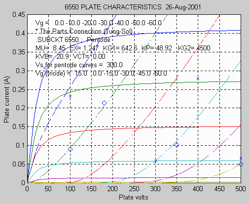
The following text is displayed in the Matlab window. It should be selected, cut and pasted into your tube model library (filename.LIB) using a text editor (the Matlab editor or Wordpad work fine). Capacitances should be added manually following the line starting with + KVB. I recommend adding around 1 pF to the published capacitances for the tube socket and wiring. The remainder of the lines in a tube model are illustrated in Improved vacuum tube models for SPICE simulations, part 2.
The 12AX7A triode: 12AX7AMitch.m.SUBCKT 6550 1 2 3 4 ; P G1 C G2 (Pentode)
+ PARAMS: MU= 8.45 EX= 1.247 KG1= 642.5 KP= 48.92 KG2= 4500
+ KVB= 20.9 VCT= 0.00
* The Parts Connection (Tung-Sol) 25-Aug-2001
.ENDS
TubeName = '12AX7A';
Source = 'Tom Mitchell';
axset = [0 400 0 .006]; MU = 100;
VGP = 0:-.5:-3; Vpmax = 400;
Vp = [100 250 200 300 300 360];
Vg = [0 0 -1.5 -1.5 -3 -3];
Idata = [.00194 .00652 .00091 .00318 .00040 .00128];
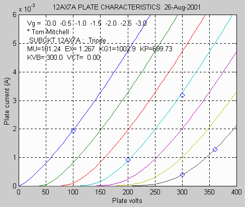
Text from Matlab window (see notes under 6550):
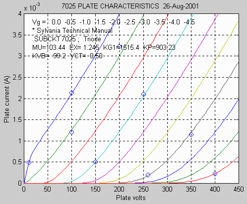
The 7025 triode (similar to the 12AX7), illustrating contact potential (VCT): 7025.m.SUBCKT 12AX7A 1 2 3 ; P G C (Triode)
+ PARAMS: MU=101.24 EX= 1.267 KG1=1002.9 KP=699.73
+ KVB= 300.0 VCT= 0.00
* Tom Mitchell 26-Aug-2001
.ENDS
TubeName = '7025';Text from Matlab window (see notes under 6550):
Source = 'Sylvania Technical Manual';
VGP = 0:-.5:-4.5; Vpmax = 450; VCT = .5;
axset = [0 450 0 .004]; MU = 100; KVB = 7; KP = 800;
Vp = [10 100 100 200 150 250 260 350 400];
Vg = [0 0 -.5 -.5 -1.5 -1.5 -3 -3 -4.5];
Idata = [.00049 .00213 .00121 .00323 .00050 .00210 .00020 .00115 .00022];
7025 plate characteristics, illustrating contact potential (0.5 V)
.SUBCKT 7025 1 2 3 ; P G C (Triode)
+ PARAMS: MU=103.44 EX= 1.245 KG1=1515.4 KP=903.23
+ KVB= 99.2 VCT= 0.50
* Sylvania Technical Manual 26-Aug-2001
.ENDS
| This page was created in 2001. Images and text copyright (C) 2000-2012 by Norman Koren. Norman Koren lives in Boulder, Colorado. Since 2003 most of his time has been devoted to the development of Imatest. He has been involved with photography since 1964. Designing vacuum tube audio amplifiers was his passion between about 1990 to 1998. |  |